Raster Grids

Raster grids are also referred to as a TIN (triangulated irregular network), Grid Image, Raster Image or a Surface.

A raster image can take many forms, such as .bmp, .tif, .jpg etc. If you examine a raster image closely you notice that they are made up of many (usually) square cells. In a raster GIS, these cells are used to represent geographic data. Every cell contained in the raster map also has either numeric or character attribute information associated with it.

A raster based GIS can portray continuously varying data more effectively and can analyze multiple layers of data easily. Raster GIS is relatively fast and you can perform a wide range of visualization and analysis that are not possible in a vector based system.

Generally the cell values are referred to as a “Z” value and represent any type of numerical or character data; such as elevations, assays, rainfall, integer class codes for vegetation or lithology types, solar flux, trace element concentration, geology etc.

Note: MapInfo Pro is limited to display square grid cells, and the cell edges must be orientated parallel to the coordinate system (projection) grid North axes.

The colour of each cell is calculated based on the value of the cell, and a colour look-up table. A Raster Grid can have multiple values or attributes per cell, these are referred to as Bands, this grid would then be referred to as a multi-banded grid.

Common datasets stored in surface grids include:

• Elevation data (DEM/DTM) - this maybe raw or interpolated data.
• Interpolated geochemical or geophysical data.
• Remotely sensed data (which includes multi banded spectral satellites such as LANDSAT or SPOT).

Creating Raster Grids and Raster Grid Interpolation

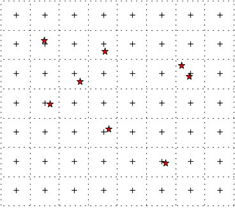
A number of interpolation methods are used to create Raster Grids from attributed points. Some methods are designed for equally spaced data with smooth changes between points values; other methods are better designed to handle disperse or clustered point datasets. In the image below the input data points (red stars) are seen with a surface grid mesh overlayed (dashed boxes).

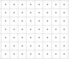
Surface grid creation does not directly assign the input data point value into the grid mesh (this is called stamping). Rather an estimate (interpolation) is calculated at each centre from the surrounding input data. The image below shows a final raster grid created with cell centres.

Steps to create a surface grid include:

1. Read input data point values.
2. Setup surface grid geometry (mesh), so the centre XY points are known for each cell.
3. At each cell centre apply interpolation (gridding) method to determine a cell value. This requires the application of an interpolation to the input data points that are closest to the cell centre.
4. Save the grid file containing the interpolated (estimated) values at each cell centre.

Grid Geometry

To determine the geometry of a grid three parameters are required:

1. Grid cell size.
2. Grid bounds.
3. Number of rows/columns (automatically calculated by dividing the bounds by cell size). A general rule to apply when determining cell size for evenly spaced data is half the mean distance of the input data points. This is to ensure only one data point is used to interpolate each cell, so resolution is not lost.

For clustered or disperse input datasets, you need to make a judgement call based on the geometry and location of the input datasets. For example, multiple grids may need to be created to correctly interpolate the dataset.

Raster Gridding Methods

Triangulation Gridding Method

The triangulation gridding method performs a Delaunay triangulation with linear interpolation. The method works by first triangulating the input data into a TIN mesh. It then calculates a value at the centre of each cell in the output grid using linear interpolation from the triangle that overlaps with coordinate of the centre of each grid cell. In order for the software work with huge datasets that could potentially contain billions of triangles on PCs with limited available memory, the input data is scanned, spatially sorted and divided into tiles. Each of the tiles is then triangulated and the resulting TIN mesh is either stored in memory or if there is insufficient memory available it is stored on disk in temporary files. Once the dataset has been triangulated into a TIN mesh the output grid is constructed by interpolating cell values from the triangles.

Because the triangulation process is relatively autonomous it is possible to leave the gridding properties set to their default settings and the software attempts to automatically compute an appropriate set of parameters for the output grid by examining the field and spatial statistics of the input file(s). If you are unfamiliar with the distribution or range of the input data sets then leaving the gridding properties on their default settings is recommended.

If you are familiar with the input dataset and know in advance what the spatial extents and distribution of the data is like and you have a good understanding of the range of values in the field(s) being gridded then you can manually adjust the gridding properties to suite the input and output data requirements.

Triangulation properties

The triangulation properties can be used to influence the geometry of the data structures, the number of points and memory that is used to triangulate each tile of input points.

Maximum Triangle Side Length

This parameter applies to the triangulation phase of gridding and can be used to minimize or eliminate long thin triangles that may be created across large holes or gaps in the data or between widely separated points that lie around the perimeter of the dataset. By default triangles that are created with a length that is greater than half the diagonal length of a tile is discarded. The size of the tiles used during triangulation are determined automatically by the software after it analyses the spatial statistics of the input points, however you can modify the size of the tiles by applying a Triangle patch multiplier.

Distance Specified in Data Units

This parameter is used to control the units of distance that the Maximum triangle side length property is measured in. By default this control is disabled and the maximum distance unit is expressed as a ratio of the tile (or patch) size. If you wish to constrain the Maximum triangle side length to a fixed value that is measured in absolute data units (e.g. 100 m) then enable this control and enter in the appropriate value. If the entered value is large and exceeds the size of an individual tile of data then it may have no effect on the output grid.

Note: If the coordinate system of the input data is Longitude/Latitude then the absolute distance units need to be specified in fractions of a degree (Arc seconds).

Triangle Patch Multiplier

The triangle patch multiplier can be used to modify the number and size of tiles (or patches) that the software segments the input data into before sequentially triangulating it. The tile size is automatically determined by the software following a detailed analysis of the spatial statistics of the input data. Under special circumstances the patch size can be modified by applying a Triangle patch multiplier. Increasing the default value of 1 to a higher number creates larger patches and may assist in the infilling of large holes or gaps in the dataset, however it also increases peak memory usage during the gridding phase. For very large datasets increasing the Triangle patch multiplier reduces the number (but not the storage requirements) of temporary files that are created during the gridding phase. For most datasets a patch multiplier of 1 or 2 is sufficient. Increasing the patch multiplier beyond a value of 4 would be rarely necessary.

Inverse Distance Weighting (IDW)

Inverse Distance Weighting (IDW) is a universal technique that can be applied to a wide range of spatial data. IDW uses weighted average interpolation to estimate grid cell values and can be used as either an exact or a smoothing interpolator. Each grid cell value in an output surface is calculated using a weighted average of all data point values that lie within a specified search radius surrounding the grid cell. The IDW method is optimal when the data has a fairly uniform distribution of input points across the area to be gridded, and some degree of smoothing is beneficial.

In order for the software work with huge datasets that could potentially contain billions of points on PCs with limited available memory, the input data is scanned, cleansed and stamped into a temporary grid. The grid is then divided into tiles and each tile is then interpolated using the IDW algorithm. The intermediate grids are either stored in memory or if there is insufficient memory available they are stored on disk in temporary files. Once the dataset has been interpolated the output grid is constructed by stitching together the interpolating tiles into a continuous grid.

Before commencing a gridding operation it is important that the IDW Properties are appropriately configured for the input dataset. If you are familiar with the input dataset and know in advance what the spatial extents and distribution of the data is like and you have a good understanding of the range of values in the field(s) being gridded then you can manually adjust the IDW properties to best suite the input and output data requirements.

Inverse Distance Weighting Properties

The model parameter controls the weighting model that is used to average the data points that are located within the search distance radius. The following four weighting models are available:

• Gaussian—The weight assigned to each input value is determined according to a 2D Gaussian function centred on the grid node. The shape and standard deviation of the Gaussian function is proportional to the Range value. Larger range values produce flatter functions Gaussian functions and a smoother grid. The Nugget, Range and Distance radius values are measured in increments of the output grid cell size.
• Linear—Each input point's weight is proportional to its Euclidian distance from the grid node being interpolated. The linear weight model enables the Nugget and Range parameters to be adjusted in order to vary the weight assignments. At distances less than the Nugget distance the weight model is 1 (i.e. all data contributes equally). At distances beyond the nugget value the weighting factor is applied according to the selected model. The Range parameter is used to set the outer distance threshold for which the weight model is applied. Any samples which exceed the Range and are less than the Distance radius is assigned an equal weight. The Nugget, Range and Distance radius values are measured in increments of the output grid cell size.
• Exponential—Each input point's weight is proportional to its Euclidian distance from the grid node being interpolated raised to the specified power. Increasing the power value causes smaller weights to be assigned to closer points and more distant points to be assigned equal but large weights. Increasing power values causes each interpolated grid node to more closely approximate the sample values closest to it. As with the Linear model the Nugget and Range properties can be modified to constrain that distance over which the exponential weight model is most effective.
• Power—The default option, each input point's weight is proportional to the inverse of its distance to the specified Power from the grid node. Increasing the weighting power reduces the influence distant points have on the calculated value of each grid node. Large power values cause grid cell values to approximate the value of the nearest data point, while smaller power values results in data values being more evenly distributed among neighbouring grid nodes. The weighting value defaults to 2 (i.e. the weight of any data point is inversely proportional to the square of its distance from the grid cell) which is appropriate for most situations. If required, the weighting value can be altered to any positive value.
• Distance Radius—It is important to set an appropriate size for the search distance radius. Setting it smaller than the average data spacing may result in a large number of the interpolated grid cells being assigned a null value and therefore displayed as transparent in the output grid. Conversely, if the search distance is set to be too large then significant grid smoothing or artefacts may occur. The search distance radius is measured in increments of the output cell size.

  To optimize performance, choose a search radius that is likely to encompass the minimum number of required input points most of the time. It can sometimes be very difficult to make this decision but a good rule of thumb is to keep the search distance to a value less than or equal to 5x the output cell size.

• Distance Taper—Taper controls allow you to apply a taper function to the interpolated value of each grid node based on its distance to the nearest valid sample point. The taper function is applied using a linear weighting model thereby adjusting the expected grid node values towards the background value. Between a distance of zero and the NEAR distance the taper function is assigned a constant value of 1 (i.e. no modification is made to the grid node). Between the NEAR and FAR distance the taper function is applied as a linear weighting between the grid node value and the background value. Beyond the FAR distance grid nodes are assigned the background value.

Minimum Curvature (Full and Stamped)

The Minimum Curvature gridding method is widely used in many branches of science and research. This method creates an interpolated surface similar to a thin, linearly elastic plate passing through each of the data values defined in the input dataset. An important criterion in creating a surface is that it has a minimum amount of bending forced upon it to conform to the data points. The degree of bending is constrained by a percentage change tension parameter. Minimum curvature gridding generates the smoothest surface possible while attempting to honour the data as closely as possible. Like all gridding methods, minimum curvature gridding is not an exact interpolation technique and therefore some error may occur between the input data point values and the interpolated surface values.

Minimum Curvature (Full and Stamped) Properties

The minimum curvature (full and stamped) properties can be used to influence the geometry and smoothness of the output grid file

Stamping Method

This parameter controls the accumulation rules that are applied when multiple data points fall within a single grid cell. There are several options available:

• Average all—(last in weighted): averaged all data points.
• First Only—The first point value is assigned to the cell. All subsequent points are discarded.
• Last Only—The last point value is assigned to the cell.
• Average All—Averages all coincident point values.
• Average All (inverse distance weighted)—Averages all coincident points by applying an inverse distance weighting function.

Radius

The radius control defines a distance radius around a grid cell to search for valid input points. Distance is measured in increments of the output grid cell size.

Clipping

The clip control provides a number of options for clipping the extents of the interpolated grid, so that it more closely approximates the distribution of the input data. Options available include:

• None—No clipping is applied to the output grid. With none selected the entire output grid is filled with interpolated values.
• Near—The Near value represents the distance, in cell size increments, that the grid is to be clipped back to from the convex hull of the data points. Areas in the grid which lie beyond the Near distance is assigned null.

  Note: Setting a Near only clip value has the same effect as setting a buffer clip distance.

• Near and Far—The Far distance is the maximum distance for which interpolation occurs between input points. Any area in the grid that has data points greater than the Far distance value is displayed as null.

Full minimum curvature vs stamped minimum curvature methods

Although the operational phases for these methods appear to be very similar, there are important processing and operational differences between the two techniques. It is important to consider these differences carefully when deciding which gridding method to use. The primary operational difference between the stamped minimum curvature and full minimum curvature methods is that the stamped method is faster and requires less hardware resources (disk space memory and processing power) than the full minimum curvature method. The stamped minimum curvature method is generally faster because it does not spatially sort or retain a full temporary copy of the input data during phase 3.

Instead it stamps the input data directly into a temporary grid. In contrast the full minimum curvature method spatially sorts and stores a complete temporary copy of the input data in addition to stamping the points into a temporary grid. The two methods also differ during the final interpolation phase where the full minimum curvature gridding operation loads the spatially sorted temporary data again to complete the interpolation. Loading the data a second time requires additional processing time.

The additional performance cost incurred by the full minimum curvature algorithm is often rewarded in terms of better grid quality and estimation accuracy. The method is able to produce a better estimation for grid cells that contain one or more input data points. In comparison the stamped method may simply shift the data values to the centre of each cell (depending on the data accumulation methodology selected). The full method is able to make a better estimate of the cell value in these cases by taking into account the actual position of the input data value(s) rather than just the cell centre which may improve the estimates for all surrounding grid cells.

Due to the potential improvement that the full minimum curvature method offers in output grid quality it is the recommended method, except where you determine the improvement in the grid quality is not be detectable or significant, or that the additional processing cost is too high.

The stamped minimum curvature method may be more appropriate in the following situations:

• Re-interpolating existing gridded data onto a finer mesh. If the fine mesh is carefully designed so that the centre of the existing grid cells always fall in the centre of the cells of the new grid, then stamped minimum curvature returns the same result as the full method. However, if the cells are non-aligned then the full method produces a better result.
• The output grid cell size is very small compared to the input data spacing. As a guideline if the grid cell size is 8x to 10x smaller than the input data spacing. In this case the input data value is close to the centre of the cell into which it is stamped.
• The output grid cell size is large compared to the input data spacing. As a guideline if the grid cell size is 2x larger than the input data spacing then you are more likely to want the grid cell estimation to represent the average value of the observations within the cell.
• Noisy data. If the input data has a high level of noise then there is little reason to more accurately represent it by using the full minimum curvature method.
• Large data measurement footprint. If the data observations represent an average of a large footprint (e.g. radar) then stamped minimum curvature may be sufficiently accurate. However, where the observations represent an accurate point measurement of a smooth continuous field then full minimum curvature should always be used.

Data Density

The Density gridding method produces a grid which records a measure of the point density at each grid node. The density at each grid node is determined independently using a kernel estimator function.