PTCLD2WF Process
To access this process:
-
ribbon
-
Solids ribbon >> Create >> Point Cloud Solid
See this process in the Command Table .
Process Overview
PTCLD2WF reconstructs surface data files from input point cloud files.
A single input points file containing surveyed point data is expected. Point density and arrangement can be uniform or irregular. Points can optionally be declustered and, if normal calculation is required, these stages can be performed independently of surfacing or as one combined operation, depending on @RUNMODE.
PTCLD2WF processing involves up to 3 phases, depending on the wireframe surfacing method chosen:
-
Input points are declustered to decrease point density and encourage a more uniform point layout.
-
Input point data is appended with normal information, indicating the normal direction to be considered when specific surfacing methods are used. Not all methods require point normal calculation.
Normal data can also be extracted from the input points file if it is present.
-
A surface is interpolated between points using a combination of surface method and appropriate parameters.
In all cases, the input file is a Datamine (.dm) points file and the output files are a wireframe file pair.
Note: PTCLD2WF parameters may be dependent on other settings. For example, @DEPTH, @WIDTH, @SAMPNODE, @PTWEIGHT and @BOUNDTYP are only used if @WFMETHOD is 1 or 2. Similarly, if @WIDTH is greater than zero, @DEPTH is not used.
Another example: if @WFMETHOD is not 1, @BOUNDTYP is not used.
Declustering Raw Point Cloud Data
Raw point cloud data can be denser than required for a suitable surface reconstruction.
Declustering options are:
-
Random point removal (to achieve a target @SSDIST value). This is @SSMETHOD=1.
-
To achieve a target @SSDIST distance between points. This is @SSMETHOD=2.
-
To decluster to a specific octree depth, again provided by @SSDIST). This is @SSMETHOD=3.
See DECLUST.
Computing Point Normals
Point normal computation relies on the following parameters: @NNEIGHBS and @RADIUS. An explanation of these parameters can be found in the table further below.
Point normal computation is only required if @WFMETHOD is either 1 or 2. Surface reconstruction will not complete if either method is specified and point normal data is not available. If @WFMETHOD is anything other than 1 or 2, all point normal computation parameters are ignored.
Point normals can be computed for any input point data, either as an independent task (@RUNMODE=2) or as part of the full surface reconstruction process (@RUNMODE=4). Alternatively, if normal data is already available for the input point cloud, *NORMALX, *NORMALY and *NORMALZ can be mapped beforehand.
Note: If normal attributes are specified but a run subsequently includes normal computation (e.g. @RUNMODE is either 2 or 4), computed normals will be used in preference to mapped fields.
Point Reconstruction Surfacing Methods
PTCLD2WF supports 5 different surface reconstruction methods. Some require point data to include normal directions and some, which perform a Delauney triangulation, don't.
Which method is suitable for your data depends on a range of criteria, including:
-
Point data pattern regularity.
-
Point data density and the extent of declustering required.
-
Extent of data 'noise', that is, errant points generated by data collection or preprocessing.
-
The general shape implied by a point cloud (e.g. a primitive-like cavity shape, such as a stope may require a different surfacing method to a grid of development drives, cubbies and so on.
-
Absolute point-to-surface adjacency requirements.
-
Processing time requirements.
@WFMETHOD=1
This method reconstructs a surface by solving a Poisson system (solving a 3D Laplacian system with positional value constraints). This method requires normal data to be associated with input points. Data that implies a relatively simple, singular mass, where data points are relatively evenly distributed, are often good candidates for this method. As an interpolative method, the generated surface may not lie precisely on all input points, instead forming a trend between points in 3D space.
This method cannot process point data without normal specifications. This method supports the widest range of surface generation parameters; @DEPTH, @WIDTH, @SAMPNODE, @PTWEIGHT and @BOUNDTYP.
@WFMETHOD=2
Reconstructs a surface by solving for a Smooth Signed Distance function (solving a 3D bi-Laplacian system with positional value and gradient constraints). Can be moderately more accurate than Poisson option but may also take longer. Data that implies a relatively simple, singular mass, where data points are relatively evenly distributed, are often good candidates for this method. As an interpolative method, the generated surface may not lie precisely on all input points, instead forming a trend between points in 3D space.
The following parameters are supported for surface reconstruction; @DEPTH, @WIDTH, @SAMPNODE and @PTWEIGHT.
@WFMETHOD=3
Reconstructs a surface using a Delauney triangulation method and will generally produce a watertight volume. This method doesn't require (or use) any process parameters and any parameter settings are ignored. Input points data can be of any arrangement and, whilst interpolation is minimized, point-to-surface adherence may still be inexact in places of sharp directional changes.
@WFMETHOD=4
Reconstructs a surface using a Delauney triangulation method by simulation the path of a ball rolling across the input data. The only parameter used by this method is @RADIUS which determines the radius of the rolling ball (with higher values tending to produce more general shapes).
@WFMETHOD=5
Reconstructs a surface using a fast advancing front method. It can be useful for a rapidly generated initial data preview, particular where input data is dense. It's very quick, but may be imprecise. Recommended for an initial shape preview.
Parameter Suggestions
The arrangement of points in 3D space resulting from underground scanning and monitoring systems is infinite. A surface reconstruction calculation involves interpolating the most appropriate 3D surface between those points. To achieve a satisfactory result, some guidance can be offered in the form of additional parameters. PTCLD2WF
The following examples may help you decide reasonable starting parameters for your point reconstruction scenario.
Banded CMS Data from Fixed Origin
This example relates to data captured from a fixed CMS, resulting in fan of survey points originating from strings of a common origin, captured at regular dip changes. For example:
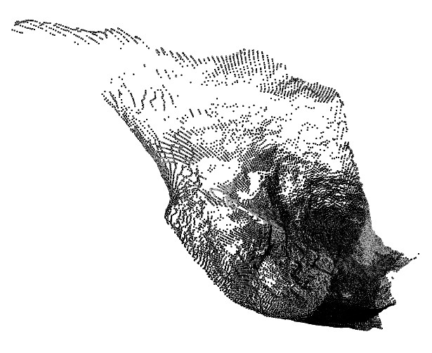
In this case, data density varies across the data (dense at the origin and less so at distance). This variation in density tends to make interpolated solutions struggle; the large gaps at distance from the monitoring tool can be misconstrued as air, breaking the resulting wireframe up. A triangulated solution, such as @WMETHOD=3,4 or 5 is likely to generate a more natureform result.
Regularly-spaced CMS Input
This example relates to a cavity scan resulting in a dense, uniformly separated points in a grid arrangement.
In this case, the level of interpolation required is relatively low (points are never that distant from other points). As such, a Poisson (1) or SSD (2) solution is likely to provide a good result, as will Delaunay triangulation methods (3, 4 or 5).
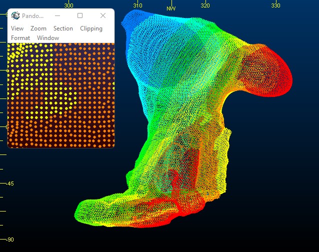
If you're going for complete point adherence (=100% data accuracy), a triangulation method may be more appropriate, but if you want to ignore outlier or aberrant data and produce a more general (potentially smoother) result, an interpolative approach my be better in this case.
"Banded" Lidar Scan Data
In this example, scanned points are derived from a mobile LIDAR rig, with data captured at regular intervals along a series of drives.
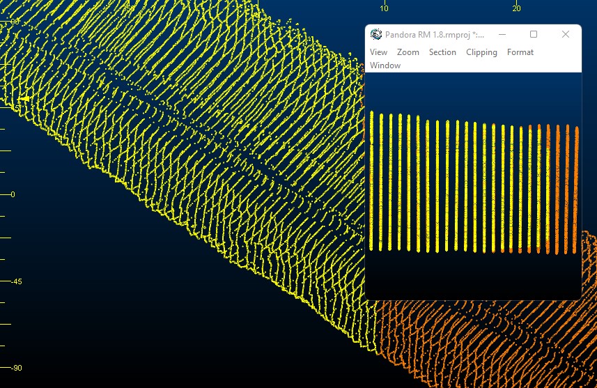
This data arrangement presents a particular challenge as each 'band' of points contains very closely-spaced points, but the gap between each band is significantly wider than those within each band. A Delaunay method (@WFMETHOD=3,4 or 5) will often yield good results in this case as methods 1 and 2 calculate an interpolated solution between points (based on the normal direction of neighbouring points) and, because the point spacing in the data is in two very different ranges (in the bands and between the bands), a single set of parameters for interpolation can produce less accurate results.
Regular but Incomplete Data
Fixed monitoring systems can capture incomplete scenarios due to data 'shadowing' caused by obstacles within the capture zone.
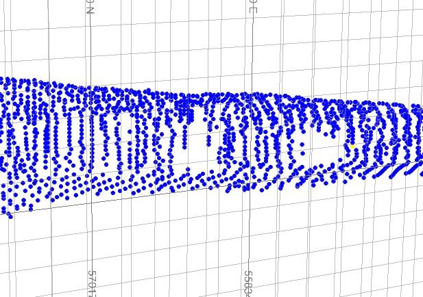
In this situation, @WFMETHOD 1 or 2 with a relatively high @PTWEIGHT (<10) may help to close unwanted gaps whilst still honouring the trend of the data. This is because points will influence surface generation out to a greater distance than if @PTWEIGHT were arbitrarily low. A triangulated approach (methods 3,4 or 5) would simply bridge the gap using straight edges, which may be fine for small gaps but not for larger ones.
Point Reconstruction - Tips
The huge range of possible point file configurations makes it difficult to provide fixed rules for surfacing data, but the following general rules may help you get a good start with your reconstruction task:
-
Declustering can reduce input points and even encourage a more regular arrangement. It can significantly improve processing times. The downside is that declustering removes real world data and could be at the cost of accuracy. Declustering can be performed regardless of the surface reconstruction method.
-
Review your declustered (".._SS.dm") and normal-appended ("..._N.dm") points in the 3D window to see how declustering and normalization is performed for a run.
-
@WFMETHOD = 5 is the simplest, and is also the quickest. Start with this method to preview how simple triangulation is performed, and decide if an interpolative technique is required instead.
-
If you just want to surface between points, without any interim interpolation or trend analysis, @WFMETHOD 3, 4 or 5 are ideal. They are also very quick to complete and, other than method 4 (which requires a ball radius parameter) the only specifications required are the file to be processed and the name of the processed file.
-
@WFMETHOD 1 and 2 rely on interpolative techniques (solving a 3D Laplacian system). These can take longer to complete than the other methods, but will consider data and its surrounding points to generate a surface along an implied trend. This can be useful where data is regularly spaced, but incomplete.
-
If using @WFMETHOD 1, if @BOUNDTYP is set to 2 (a Direchlet boundary system), the output is likely to be a watertight volume. @WFMETHOD 3 is also likely to produce a closed volume.
Input Files
|
Name |
Description |
I/O Status |
Required |
Type |
|
IN |
Input point cloud data file used to create the wireframe surface. |
Input |
Yes |
Points |
Output Files
|
Name |
Description |
I/O Status |
Required |
Type |
| POINTS | Output file prefix for subsampled points and points with normals. A file containing subsampled points will have an _SS suffix. Points with normals will have a _SSNORM suffix. This must be specified if @RUNMODE = 1,2 or 4. | Output |
Yes, if @RUNMODE=1, 2 or 4. Otherwise, no. |
Points |
| WIRETR | Output surface wireframe triangle file. | Output | Yes | Wireframe Points |
|
WIREPT |
Output surface wireframe point file. |
Output |
Yes |
Wireframe Triangles |
Fields
|
Name |
Description |
Source |
Required |
Type |
Default |
|
X / Y / Z |
Name of X/Y/Z coordinate field in *IN. |
IN |
Yes |
Numeric |
Undefined |
|
NORMAL X/Y/Z |
Name of X normal field in input file IN. Only used if @RUNMODE = 3 (calculate surface) |
IN |
No |
Numeric |
Undefined |
|
RED |
Name of red colour field in input file IN. Only used if @WFMETHOD is 1 or 2. |
IN |
No |
Any |
Undefined |
|
GREEN |
Name of green colour field in input file IN. Only used if @WFMETHOD is 1 or 2. |
IN |
No |
Any |
Undefined |
|
BLUE |
Name of blue colour field in input file IN. Only used if @WFMETHOD is 1 or 2. |
IN |
No |
Any |
Undefined |
Parameters
|
Name |
Description |
Required |
Default |
Range |
Values |
|
RUNMODE |
Specify the functions for the process to execute:
|
Yes |
1 |
1,4 |
1,2,3,4 |
|
SSMETHOD |
The method to use for subsampling.
|
Yes if @RUNMODE=1 or 4, otherwise no. |
2 |
1,3 |
1,2,3 |
| SSDIST |
A parameter controlling the extent to which subsampling is performed and depends on the chosen @SSMETHOD.
|
Yes if @RUNMODE=2 or 4, otherwise no. | 0.5 | Undefined | Undefined |
| NNEIGHBS | The number of neighbours used when orienting the normals using a spanning tree. Normals are not required if @WFMETHOD is 3,4 or 5. |
No unless: @RUNMODE=2 or; @RUNMODE=4 and @WFMETHOD = 1 or 2 |
Undefined | Undefined | Undefined |
| RADIUS |
Where @WFMETHOD = 1 or 2: the neighborhood radius used to compute normals. The bigger the radius, the more points will be used to compute the local surface model, resulting in generally smoother normals but also in a longer process time. A value of zero will allow the program to compute a radius value automatically. Where @WFMETHOD = 4, this represents the radius of the sphere used to generate the surface by rolling across the input points. Not used if @WFMETHOD Is 3 or 5. |
Yes if @WFMETHOD = 1, 2 or 4 | Undefined | Undefined | Undefined |
| DEPTH |
The octree depth to be used in surface construction. A higher number gives greater resolution but will be slower and use more memory. Should ideally be between 4 and 24. Values larger than 10 are likely to be process intensive. This parameter is ignored if WIDTH is specified as greater than zero. Not considered if @WFMETHOD 3,4 or 5. |
No | Undefined | Undefined | Undefined |
| WIDTH |
This floating point value specifies the target width of the finest level octree cells used in surface reconstruction. If set to zero then DEPTH is used to control octree size. Not considered if @WFMETHOD 3,4 or 5. |
No | Undefined | Undefined | Undefined |
| WFMETHOD |
The method to use to construct the wireframe surface from the set of points with oriented normals.
|
Yes | 5 | 1,5 | 1,2,3,4,5 |
| SAMPNODE |
Number of samples per node during Reconstruction. This floating point value specifies the minimum number of sample points that should fall within an octree node as the octree construction is adapted to sampling density. For noise-free samples, small values in the range [1.0 - 5.0] can be used. For more noisy samples, larger values in the range [15.0 - 20.0] may be needed to provide a smoother, noise-reduced, reconstruction. Only used if @WFMETHOD is 1 or 2. |
No | Undefined | Undefined | Undefined |
| PTWEIGHT | The importance that interpolation of the point samples is given in the formulation of the screened Poisson equation. This is a floating point number. Only used if @WFMETHOD is 1 or 2. | No | Undefined | Undefined | Undefined |
| BOUNDTYP |
This integer specifies the boundary type for the finite elements used in Poisson reconstruction (WFMETHOD=1). Valid values are:
|
No | 1 | 1,3 | 1,2,3 |
Example
!START M1
# - Use !LOCDBOFF to look for files outside the local folder
# - Use local files by deleting the next line or use !LOCDBON
!LOCDBOFF
!PTCLD2WF &IN(pointcloudCMS1),
&POINTS(pointsout),
&WIRETR(comb1tr),
&WIREPT(comb1pt),*X(XPT),*Y(YPT),*Z(ZPT),@RUNMODE=1.0,
@SSMETHOD=3.0,@SSDIST=9.0,@MODEL=2.0,@NNEIGHBS=6.0,
@RADIUS=1.0,@DEPTH=12.0,@WIDTH=0.05,@WFMETHOD=2.0,
@SAMPNODE=6.0,@PTWEIGHT=10.0,@BOUNDTYP=2.0
!END