
Stereonet Analysis - Exercises
The identification of the different sets of structural features and their associated average planes and value ranges is done by viewing all the structure point data in a Stereonet Chart, contouring the poles and generating average planes for each set. A pole is the projection of the normal to a plane onto the bounding sphere. For example, the north and south poles of the Earth are projections of the normal to the equator onto the upper and lower hemispheres respectively. A Stereonet Chart can display both the pole data and a projection of the associated plane.
The following data files were used in the examples on this page
and can be found in the tutorial data folder (C:\Database\DMTutorials\Data\VBOP\Datamine):
-
_vbgtpts.dm- structure data points file -
_vb_itpitstrings.dm- open pit crest and toe strings
Load Data
To load data and create a contoured pole plot:
The procedure for loading data and creating a contoured pole plot is as follows:
-
In the Project Data control bar, click Add Existing Files to Project to add both files to the project.
-
In the Project Data control bar, locate these two files under the Points and Strings folders, then drag-and-drop them into the 3D window (to load the files into memory).
-
Expand the 3D >> Points folder and double click _vbgtpts.dm.
The Points Properties screen displays.
-
Activate the Symbols tab and djust the Scale of the symbol to 10 and click OK.
The structure points are now more visible against the pit crest and toe strings:
-
Display the Plots window.
-
Display the Manage ribbon and select Sheets >> Charts >> Stereonet.
The Stereonet screen displays.
-
Expand Loaded Data and select _vbgtpts (points).
-
In the Dip list select SDIP.
-
in the Dip Direction list select DIPDIRN.
-
in the Key Field list check that no column is selected (this will ensure that a single chart is generated).
Note: If the default dip direction and dip data column names are present in the points file, then these fields DIPDIRN and SDIP are automatically detected.
-
Click Apply to generate and display a pole projection:
-
In the Charts tab, Show/Hide group, tick Contours to add contours to the plot (the preview pane is updated automatically):
Tip: Right-click the preview pane to display a context menu which can be be used to control the displayed stereonet.
-
Display the Charts tab.
-
In the Show/Hide group, uncheck Poles and Planes and check Contours to show only the contours:
-
Check Color Map and select Hot to update the chart:
-
Check Poles to redisplay the poles alongside contours.
Stereonet Sets
To create a stereonet set:
In the following example, a set of pole data will be selected. This set will be used in subsequent exercises to determine a plane representing an average indicator for the poles within the set.
-
Display the Charts panel.
-
Uncheck all options other than Poles. No Color Map should be selected.
-
Under Grid, check Center Cross.
-
In the bottom left of the screen check Stereonet Toolbar.
-
Using the toolbar, click Add Set (Window) icon on the toolbar.
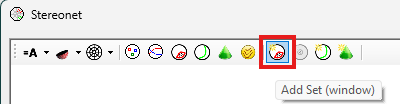
At this point, the Stereonet system enters editing mode.
-
Click once to define the 'corner' of the net segment nearest to the centre cross.
-
Move the mouse to define the opposite corner of the segment, furthest from the centre cross, for example:
The New Set screen displays.
-
Enter the name "JointSet1".
-
For the other parameters, edit the values to match those shown below:
-
First Point Dip – 50
-
First Point Dip Direction – 29
-
Second Point Dip – 13
-
Second Point Dip Direction – 61
-
Display – Average Pole, Average Plane
-
-
Click OK to display the set boundaries, average pole (for the set) and average plane (for the poles within the set):
-
Display the Sets tab.
One entry is visible in the table at the top of the screen:
-
Under Display, change the Color to green.
-
Set Line to 3:
-
Change the Average Plane Color to red, and set Line Thickness to 3.
-
Change Symbol to a triangle.
-
Set Symbol Size to "15":
Fixed Planes
To add a fixed plane:
You can insert a new fixed plane if you know the dip direction and dip.
-
Select the Planes tab.
-
Click Insert Plane at the top of the screen.
The New Fixed Plane screen displays.
-
Enter the Name "NorthWall"
-
Enter a Dip of 50 and a Dip Direction of "40".
-
You can display the average plane of the specified dip and dip direction and/or the average pole position. It is also possible to display the Daylight Envelope for the fixed plane.
")
-
Check Plane, Pole and Daylight Envelope and click OK.
The stereonet chart updates:
See Daylight Envelope.
Friction Cones
See Friction Cones.
Highlight Selected Data
A key feature of your Stereonet facility is the ability to select poles within your current stereonet plot, and highlight that data in other data windows. The Stereonet screen is 'modeless', meaning other functions outside of the screen can still be accessed when it is displayed.
The Stereonet display also highlights data even when data is selected in, say, the 3D window. This means you can easily see the planar information that is contributing to the stereonet in a particular area.
To highlight specific data in Stereonet and other views:
-
Display the Stereonet screen and complete the exercise shown above under "Stereonet sets".
-
Select all poles within the previously created set ("JointSet1").
-
Right-click the in preview pane (on the left) to display the context menu.
-
Choose Selection >> Select Set.
-
Click inside the green boundary of your custom data set. All poles within it are highlighted. Any associated average plane, pole or daylight envelope indicators are also highlighted:
Tip: Change your highlight colour in System Options.
-
Move the screen aside so you can clear access the Plots window. The data within this window is also selected:
Note: the hatched effect is intentional - it indicates that the plot is currently 'under construction'.
-
Display the 3D window and select planar data to highlight it.
The corresponding stereonet chart data highlights as well.
Related topics and activities: