
MIKEST Process Example
To access MIKEST:
-
Estimate ribbon >> Non-Linear >> MIK.
- Enter "MIKEST" into the Command Line and press <ENTER>.
-
Display the Find Command screen, locate MIKEST and click Run.
The MIKEST process uses the Indicator Estimation (IE) method to estimate grades into a block model using the cumulative distribution function (CDF) of indicator transformed sample grades. It is similar to the INDEST process except it is based on the Advanced Estimation COKRIG process rather than the ESTIMA process.
Note: The main advantage of MIKEST over INDEST is processing speed.
This topic describes a worked example of using dynamic anisotropy within the MIKEST process.
MIKEST Example
This example is designed to show the files, fields and parameters that are used by the MIKEST process when using the Dynamic Anisotropy option. In order to keep file listings small only 3 cutoffs have been used whereas in practice around 12 cutoffs would be more usual. The example uses 1 zone control fields, ZONE, with 3 zone values, 1, 2 and 3.
The files used in this example are based on files available in this folder, installed with your application:
C:\Database\DMTutorials\Data\VBUG\Datamine
The above folder includes macro file DYNAM_ANISO_UG_TUTORIAL.MAC.
- Macro M1 uses digitised
plan and section strings to create
MODEL3which includes TRDIPDIR and TRDIP fields. - Alternatively, macro M2
uses wireframe data to create the
MODEL3file.
Either of these MODEL3 files can be used instead of EG1_MODEL1 in
the macro shown in the Files, Fields and Parameters section below.
SAMPLES file _VSLDHZ.DM in the above tutorials folder can be used
instead of EG1_HOLES1.DM. The results will be similar to (but
not the same as) the example files shown below.
Files, Fields and Parameters
!MIKEST &SAMPLES(EG1_HOLES1),&PROTO(EG1_MODEL1),
&EPAR(EG1_EPAR1),
&FIELDS(EG1_FPAR1),
&SPAR(EG1_SPAR1),
&VMODEL(EG1_VPAR1),
&OUTMODEL(EG1_OUTMODEL1),
&AVGRADES(EG1_AVGRADES),
&INDICATE(EG1_INDICATE),
&SAMPOUT(EG1_SAMPOUT),
*XPT(X), *YPT(Y),  *ZPT(Z),  *ZONE1_F(ZONE),
@PGFIELDS=1, @ORDER=3,  @GRMETHOD=3,
@DA_AXIS1=3.0, @DA_AXIS2=1.0,  @DA_AXIS3=2.0,
*SANGL1_F(TRDIPDIR), *SANGL2_F(TRDIP),
*VANGL1_F(TRDIPDIR), *VANGL2_F(TRDIP)
INPUT: SAMPLES FILE - EG1¬_HOLES1 - 6946 records
The field ZONE in the Samples file is used for zone control. The same field name is required in the model PROTO file. The field name ZONE is defined using the field assignment *ZONE1_F(ZONE) in the Files, Fields and Parameters section above.
INPUT: PROTO FILE - EG1_MODEL1 - 15066 records
- The parent cell size is 10 x 10 x 10
- The ZONE field is required for zone control
- TRDIPDIR and TRDIP fields are required for Dynamic Anisotropy
INPUT: ESTIMATION PARAMETER FILE - EG1_EPAR1 - 9 records
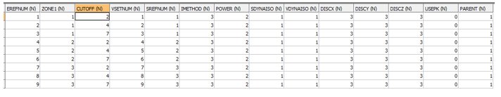
- The first zone control field in this file must be named ZONE1. It must be the same type (numeric or alpha) as the field defined by the symbolic field name *ZONE1_F() in the Files, Fields, Parameters section above. Currently only numeric zone fields are allowed.
- The CUTOFF field defines the cutoff grade for indicator calculation. Each zone must have the same number of CUTOFFs. However the CUTOFF values may differ between zones,
- The SDYNAISO field defines whether the Dynamic Anisotropy option is to be used for defining the search volume rotation angles. 0=No. 1=Yes.
- The VDYNAISO field defines whether the Dynamic Anisotropy option is to be used for defining the variogram model rotation angles. 0=No. 1=Yes.
- In this example the Search Volume Reference Number (SREFNUM) is the same for all CUTOFFs in the same zone. This is compulsory if the Dynamic Anisotropy option has been selected as only one set of dynamic search angles are stored in the input model file. It is also recommended practice if the Dynamic Anisotropy option is not selected as it helps to keep the order relation correction to a minimum.
INPUT: FIELDS PARAMETER FILE - EG1_FPAR1 - 9 records
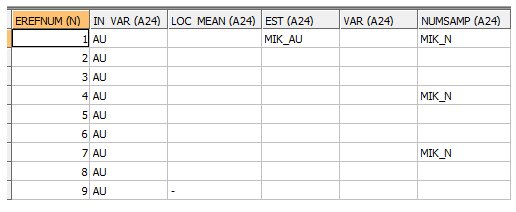
- The Estimation Parameter Reference Numbers (EREFNUM) links the field data with the EREFNUMs in the Estimation Parameter file.
- The IN_VAR field defines the grade field for which the MIK estimate is to be calculated. It must be the same for each EREFNUM.
- The EST field defines the name of the field in the output model which is to be created to define the MIK estimate. Only the name in the first record of the file is used. EST names in other records are ignored.
- The full range of optional output fields in a Fields Parameter file is available. However in this example only the NUMSAMP field has been defined to record the number of samples selected for each estimate. As the same search volume is used for all estimates within a zone it is only necessary to define it once for each zone.
INPUT: SEARCH VOLUME PARAMETER FILE - EG1_SPAR1 - 3 records

- As the Dynamic Anisotropy option is being used in this example only 3 search volumes are defined, one for each zone. The values in the SANGLE[1,2,3] fields in this file will be ignored as the dynamic search angles are defined by the *SANGL[1,2,3]_F() symbolic fields shown in the Files, Fields, Parameters section. These values will be read from the input PROTO model. Also the values for the SAXIS[1,2,3] fields shown above will be ignored as they are defined by parameters @DA_AXIS[1,2,3] instead.
- The other fields in this file are the standard search volume parameter fields.
INPUT: VARIOGRAM MODEL PARAMETER FILE - EG1_VPAR1 - 9 records
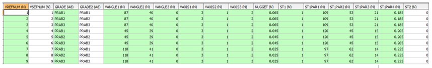
- Even though the first three variogram models are identical (same zone) they must each have a separate record as the GRADE and GRADE2 field names change. Both the GRADE and GRADE2 fields must be named PRAB1 for the first cutoff, PRAB2 for the second cutoff and PRAB3 for the third. PRABi represents the PRobability ABove cutoff i which is the name of the indicator field being estimated.
- As for the search volume parameter file the fields VANGLE[1,2,3] are ignored as the dynamic variogram model angles are defined by the *VANGLE[1,2,3]_F() symbolic fields. The variogram rotation axes are defined by the @DA_AXIS[1,2,3] parameter values.
- This example uses a single structure spherical model. Multiple structures can be used as for COKRIG.
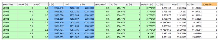
OUTPUT: MODEL FILE - EG1_OUTMODEL1 - 15066 records
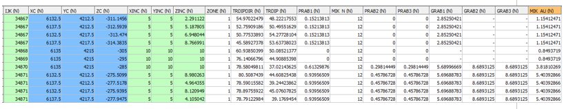
- The output model is a copy of the input PROTO model plus the last 8 fields shown above. The MIK estimate is the final field MIK_AU. As parent cell estimation has been selected all subcells within the same parent cell have the same values.
- Parameter @PGFIELDS was set to 1 so all the intermediate probability PRAB[1,2,3] fields and grade GRAB[1,2,3] fields are shown for each indicator. The first 4 subcells (IJK=34867) show that 15.21% [PRAB1] of the cells are estimated to be above cutoff 1 (2 g/t AU) but that 0% is above cutoff 2 (4 g/t). The MIK estimated grade is 1.154 g/t.
- If parameter @PGFIELDS were set to zero then the PRAB[1,2,3] and GRAB[1,2,3] fields would not be included in the OUTMODEL file.
OUTPUT: AVGRADE FILE - EG1_AVGRADES - 12 records
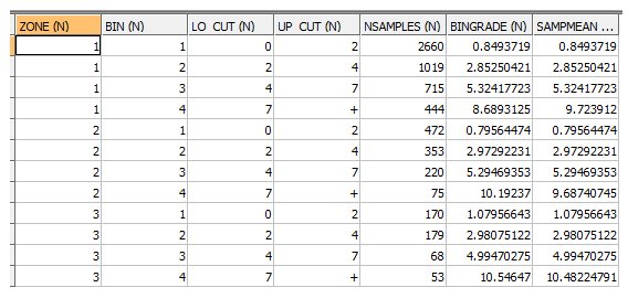
The samples are divided into 4 bins for each ZONE corresponding to the 3 cutoff grades with the 4th bin being above the top cutoff. The sample statistics are:
- NSAMPLES – the number of samples in each bin
- BINGRADE – the average grade of the samples within each bin
- SAMPMEAN – the grade used for calculation of the MIK estimate. In this example the parameter @GRMETHOD is set to 3. Therefore for the first 3 bins SAMPMEAN is equal to BINGRADE but for the top bin (bin 4) SAMPMEAN is equal to the median of the samples in the bin.
A description of all 4 values of @GRMETHOD is given in the PARAMETERS table above.
OUTPUT: INDICATE FILE - EG1_INDICATE - 6428 records
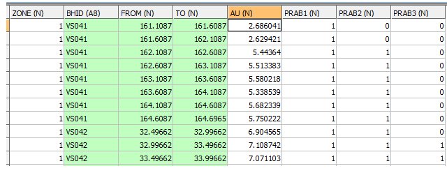
- The INDICATE file is a copy of the SAMPLES files but with a PRAB[1,2,3] value for each sample. The exception is that samples with an absent data ZONE or AU are not included. In this example 518 samples are excluded. The above table shows a subset of fields and records.
- The PRAB values depend on whether the sample is below or equal to cutoff (0) or above each cutoff (1).
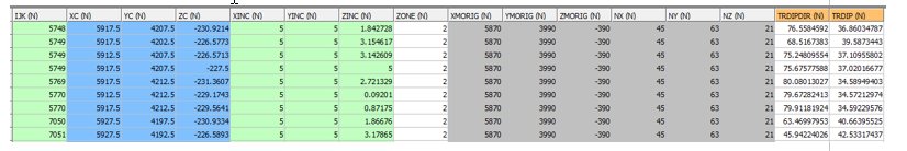
OUTPUT: SAMPOUT FILE - EG1_SAMPOUT - 213480 records
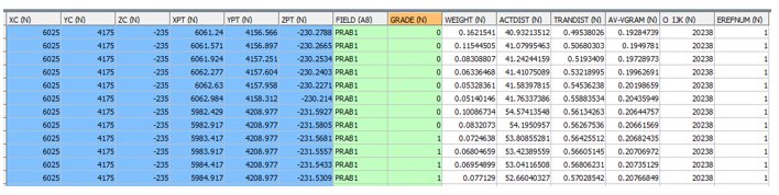
- The SAMPOUT file includes all samples used for each PRAB and each parent cell. The above subset is for the parent cell with an IJK value of 20238 (O_IJK) located at XC, YC, ZC. The FIELD name is PRAB1 so the GRADE field shows whether each sample is below (0) or above (1) the first AU cutoff (2 g/t). Other fields include:
- WEIGHT - the kriged weight
- ACTDIST – the actual (Euclidean) distance of the sample from the cell centre
- TRANDIST – the transformed distance of the sample from the cell centre based on the search ellipsoid
- AV-VGRAM – the average variogram value for the vectors connecting the sample to each discretisation point within the parent cell.
- EREFNUM – the estimation reference number as defined in the Estimation Parameter file.
Warning: The SAMPOUT file can include a large number of records. Do not select a SAMPOUT file unless you want to use it!
Related topics and activities