Configure and Apply Global Topcut Analysis

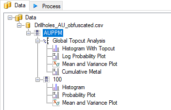
1. Insert the Global Topcut Analysis component by right-clicking the AUPPM component in the Project Tree and selecting Add » Global Topcut Analysis from the menu. Your Project Tree should now look like the image below, with the Global Topcut Analysis component and its four child components: the Histogram With Topcut, Log Probability Plot, Mean and Variance Plot and Cumulative Metal Plot.

   Note: By default, the histogram component does not have a log scale applied, whereas the probability plot does. This is in line with the disintegration method to allow for easier visualisation of the extreme values in the tail of each model. We do not recommend changing the scale type from the default settings.

   

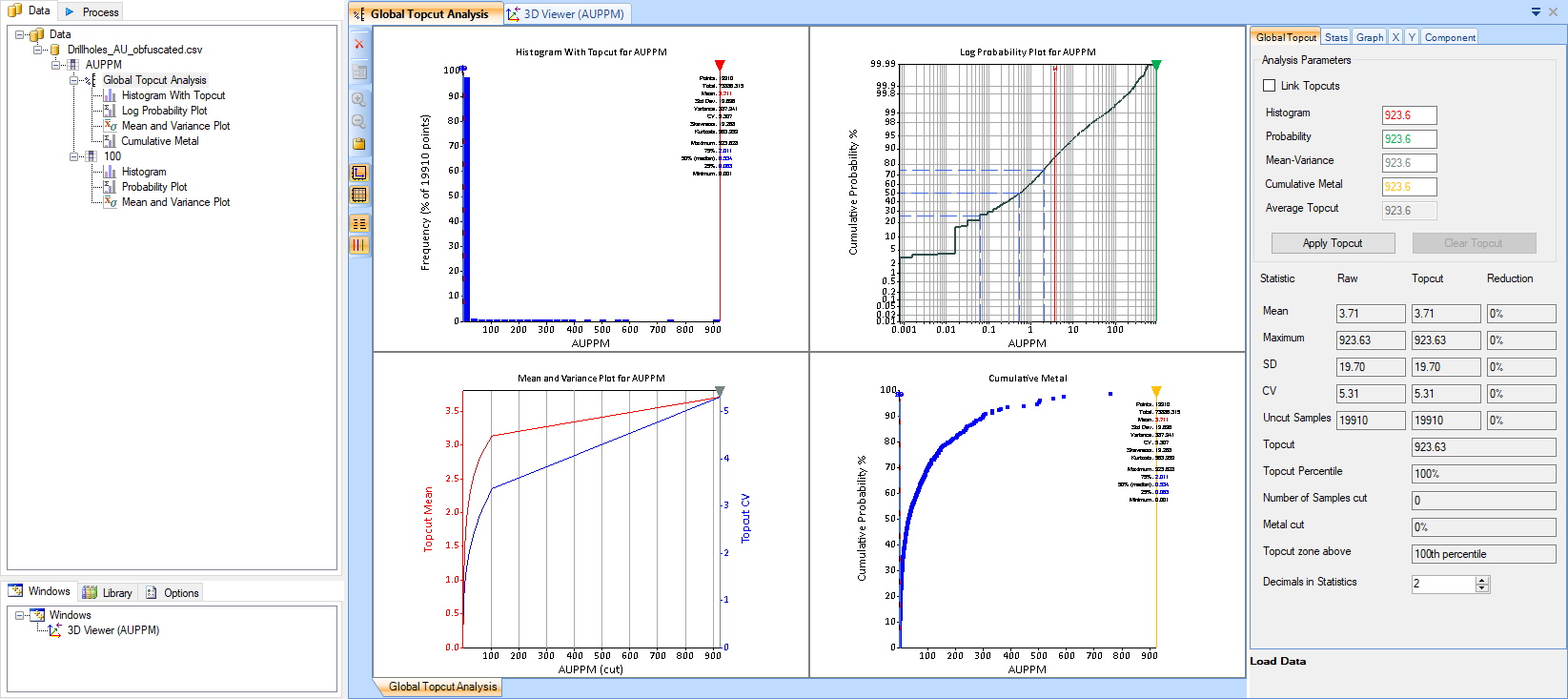
2. Select the Global Topcut Analysis component in the Project Tree to display all of the topcut components in the Main Canvas.

   When selecting the topcut value, you can either choose a value individually on each of the plots and use the average topcut value, or you can link the values and choose them simultaneously across all four plots. For this activity, we will link the topcuts.

   

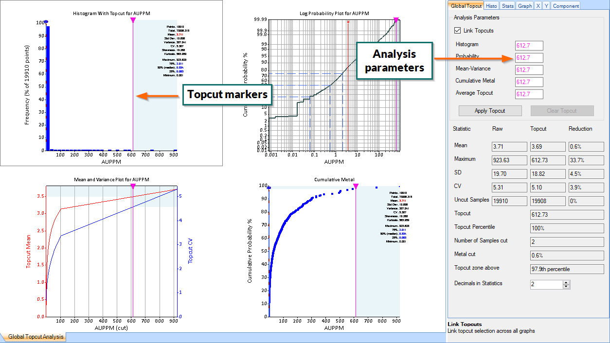
3. Check Link Topcuts at the top of the Global Topcut tab in the Property Panel.

   Note how the topcut markers and analysis parameters for each plot turn pink when they are linked, whereas they were originally each a different colour. Moving a single topcut marker when all plots are linked results in the markers on other plots moving to the same value.

   

4. To help you evaluate your data, you can adjust the axes of the histogram by clicking and dragging them. Either double-click the histogram in the Main Canvas, or click the Histogram With Topcut component in the Project Tree to enlarge that specific plot. Then click and drag the values on the Y-axis upwards to increase the size of the bars representing the tail values on the plot, as in the image below.

   

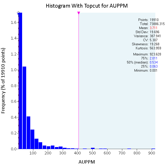
   Tip: You can reset the axes of any plot by double-clicking on the values next to the axis.

5. Return to the Global Topcut Analysis component displaying all four plots and adjust the topcuts to an appropriate value by clicking and dragging the pink topcut marker on one of the plots.

   The value that you choose will depend on the quantity and severity of the extreme values, along with the spatial context of the values within your deposit. Always incorporate your knowledge of the geology into your interpretation.

6. Use the statistics in the Property Panel to assess the number of samples cut and how this affects your data.

   In this example, the topcut value is reasonably conservative, only capping eight samples and reducing the mean by 2.1%. However, capping these samples also reduces the CV of the data by 9.8%.

   

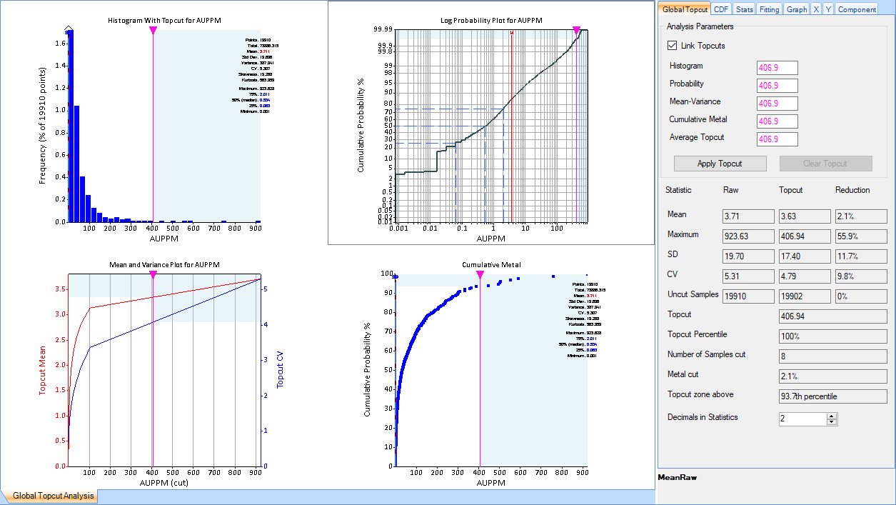
7. Once you have selected an appropriate topcut value, click Apply Topcut in the Global Topcut tab in the Property Panel.

   After applying the topcut, the new maximum value displays next to the assay value that it has been applied to in the Project Tree, as shown in the image below.

   

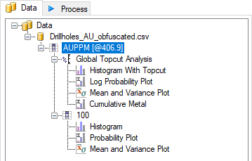
   The topcut value will be applied to all new and existing plots and analyses beneath the affected assay. The topcut can be altered at any time by following the steps above and applying a new topcut value. Alternatively, the topcut can be removed entirely by clicking the Clear Topcut option n the Global Topcut tab in the Property Panel.

«Previous