Gaussian transformation

Kriging provides the best estimate of the variable at each grid node. By doing so, it does not produce an image of the true variability of the phenomenon. Performing risk analysis usually requires to compute quantities that have to be derived from a model representing the actual variability. In this case, advanced geostatistical techniques such as simulations have to be used.

It is for instance the case here if you want to estimate the probability of NO₂ to exceed a given threshold. As in fact thresholding is not a linear operator applied to the concentration, applying the threshold on the kriged result (which is a linear operator) can lead to an important bias. Simulation techniques generally require a multi-gaussian framework: thus each variable has to be transformed into a normal distribution beforehand and the simulation result must be back-transformed to the raw distribution afterwards.

The aim of this paragraph consists in transforming the raw distribution of the NO2 variable into a normal one.

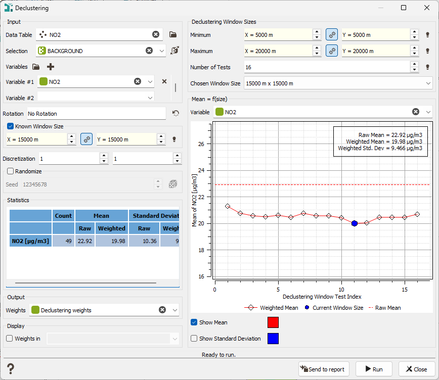
Before that, you are going to compute declustering weights. The principle of the declustering application is to assign a weight to each sample where a given variable is defined taking possible clusters into account. The weight variable which is created here may be used later in the gaussian transformation.

Click on the Data Management / Sampling / Declustering menu. Select the NO2 variable with the BACKGROUND selection and create a new variable Declustering weights. Specify the Moving Window Dimensions, i.e. the dimensions in the X and Y directions of the moving window inside which the number of samples will be counted. Generally, the average distance between the samples is taken, in your case 15 km for X and Y. The right part of the interface enables you to test different window sizes. We can a put a minimum of 5 km and a maximum of 20 km (for both X and Y) with a number of 16 tests (to test an increase of 1 km of the window size). We can see on the curve that the mean becomes constant from a size between 15 and 16 km. It confirms our original choice.

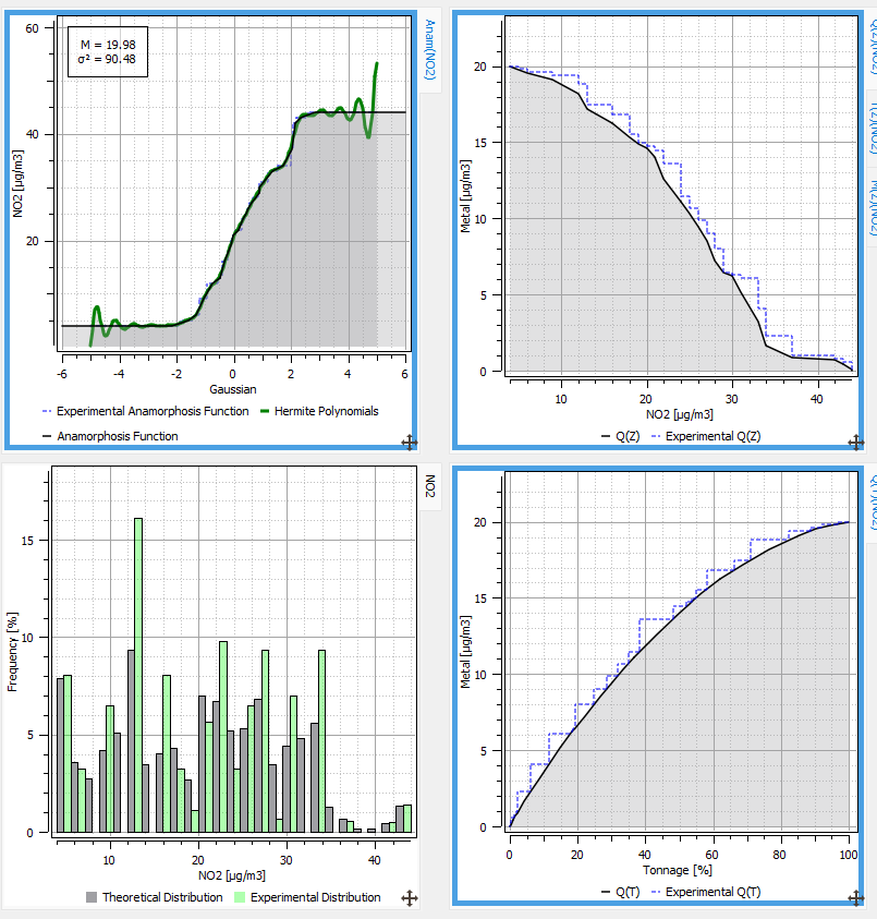
Now, using the Statistics / EDA procedure, you can fit and display the anamorphosis function.

Select the NO2 data table with the BACKGROUND selection on Input and the Declustering weights as Weights. Drag and drop the NO2 variable on the Gaussian Variables icon.

A new tab is added. The Interactive Fitting button overlays the experimental anamorphosis with its model expanded in terms of Hermite polynomials: this step function gives the correspondence between each one of the sorted data (vertical axis) and the corresponding frequency quantile in the gaussian scale (horizontal axis).

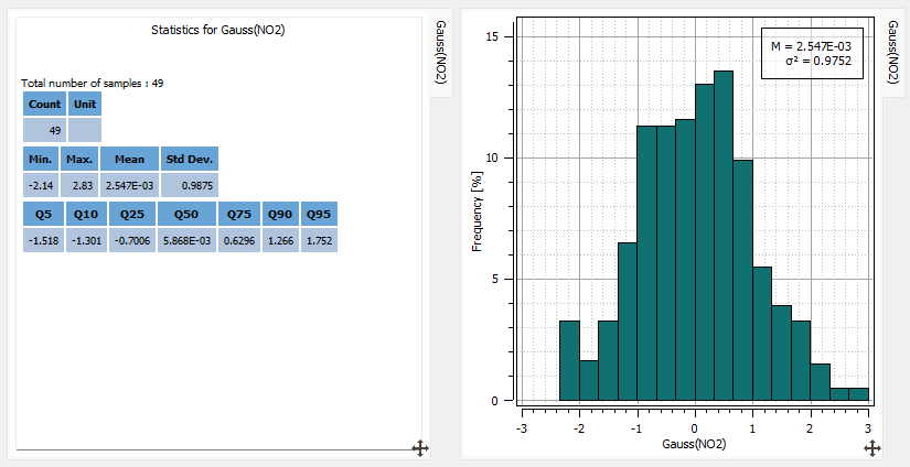
You can check the statistics of the gaussian variable by dragging and dropping the NO2 variable on the Statistics icon and defining Use the Gaussian Variable in the Variables selector in the Parameters section. These statistics take into the Declustering weights: the mean is 0.01 and the variance is 0.97.

You display the histogram of this variable between -3 and 3 using 18 classes and check that the distribution is not exactly symmetric with a minimum of -1.98 and a maximum of 2.65.

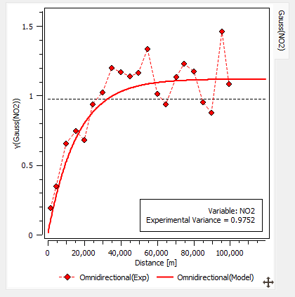
The experimental variogram calculated on the gaussian variable is very structured. The following one is computed using the same calculation parameters as in the univariate case: a lag value of 5 km and a maximum distance of 100 km.

In the Context part of the Parameters section, select Compute Gaussian Model Only in the Model Option to only see and fit the gaussian variogram. Fit a model constituted of a unique exponential structure (range 48 km and sill 1.12) and save it in the geostatistical set called NO2 (gaussian). You keep the same range as before to remain coherent. The gaussian variable, as well as the anamorphosis function are stored in the geostatistical set and will be used to compute simulations.