Presentation of the 2D Dataset

• Presentation of the 2D Dataset
• • Importing well data
  • Importing the Training Images
  • Creating the output grid
  • Exploring the data ans use Multiple point statistics with DeeSse
  • Maximum scan fraction parameter
  • Comparison with SIS
  • MPS using Multi-resolution option

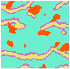
For this exercise, we provide a synthetic data set representing different meandering channels environments. It contains two Training Images corresponding to two conceptual representations of deposits with channels (a simple one and a complex one).

This dataset includes borehole locations in 2D where a categorical (indicator) variable describing geological facies is known.

There are 4 facies, identified by specific values:

• 0 = presence of flood plain deposits (this is the matrix),
• 1 = channel deposits,
• 2 = levees,
• 3 = crevasse splays.

The aim is to map the geological facies everywhere in the domain of interest represented by the simulation grid. The simulated spatial distribution of facies must be similar to the proposed conceptual models and have a realistic look of channels environment to validate the simulation.

In this exercise, we will use a multiple point statistics algorithm (DeeSse). DeeSse, as any MPS algorithm, requires a training image (TI) in addition to the borehole data. The Training Image is a reference example of the geological environment to be modelled, and the algorithm is designed to generate simulations that look like this TI. In this exercise, the TIs have been obtained by combining an object-based simulation and manual drawing to adapt the concept.

Two possible approaches will be considered and therefore two training images are provided. One of the goals of the exercise will be to evaluate which training image is the more compatible with well data.

Importing well data

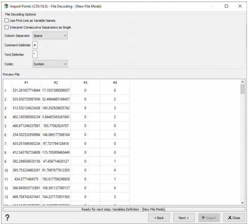
Well data containing facies codes are stored in the ASCII file hd.gslib located in the “Public” folder of the Isatis.neo project database, sub-folder “MPS 2D”. It can be loaded using the menu “Home -> CSV/XLS -> Points”. The well data is stored in a Point format.

First, import the borehole file and check the attribute table for the wells to see how the facies are coded. The attribute #4 contains the facies codes and is loaded as a numerical variable.

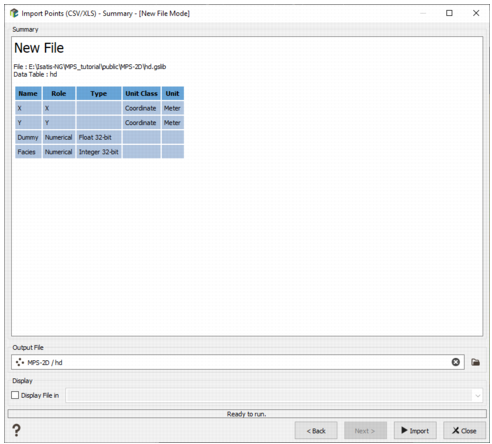
Store the loaded data in the Isatis.neo folder “MPS 2D/hd”, as shown in the figure below.

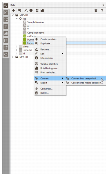
In a second step, the downloaded facies are numerical and must be transformed into a categorical variable. The simplest method for defining the categories from the numerical facies codes is to use the contextual menu Right click / Convert / Convert into Categorical in the data tree.

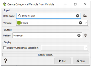
Then assign the category to the properties as shown in the figure below.

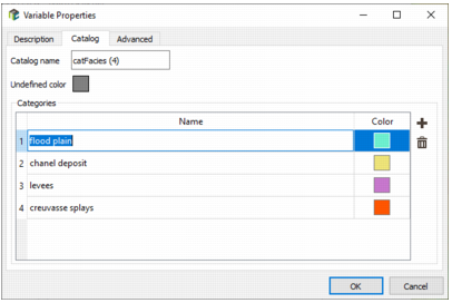
It must be noted that the automatically created categories’ names are equal to the facies codes. It is useful to replace that simple names by a geological description. Do it with the menu item Right click / Edit / Edit properties applied to the categorical variable “catFacies” stored in the Data Tree folder “MPS 2D/hd”. In the displayed pop-up window, select the tab “Catalog” and change the names as in the figure below.

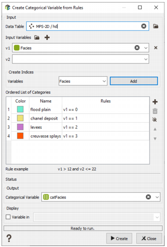
You can also do it from the menu Create Categorical Variable / From Rules.

Importing the Training Images

The Training Images are stored in the ASCII file ti.gslib located in the “public” folder of the Isatis.neo database, sub-folder “MPS 2D”. As the images have a grid structure, they can be loaded using the menu Home -> CSV/XLS -> Grid.

The grid characteristics have to be defined during the loading. They are shown in the figure below:

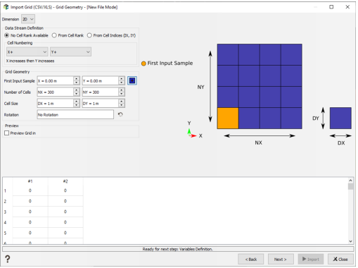
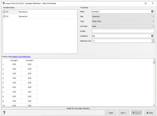
The two TI are loaded as numerical variables in this grid with the names “concept1” and “concept2”.

The two numerical variables contain the same facies codes as the well data. These variables have also to be converted into categorical variables, using the same method and the same facies names as previously.

Creating the output grid

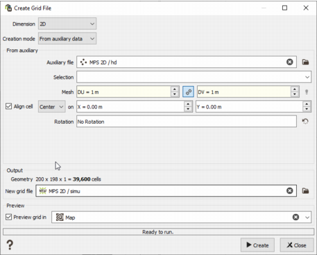
The output grid in which the simulation results will be stored has to be created. It can be done with the menu item Data Management > Create > Create Grid.

Using "From auxiliary data" as Creation mode will automatically locate the grid on the data. Select the hd points as auxiliary data.

The grid characteristics are shown in the figure below:

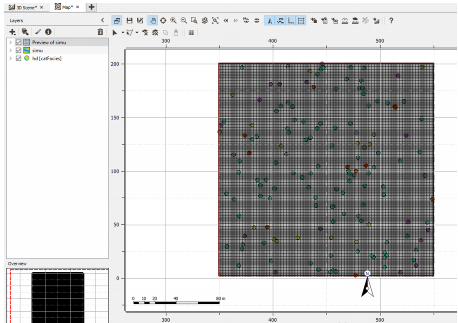
The output grid and the well data can be visualized in the Map. They should be located at the same place, like in the following image.

Exploring the data ans use Multiple point statistics with DeeSse

Look at the objects in the 3D scene (drag and drop) and use the statistics tool (right click on the object) to calculate the statistics on facies in wells and in TIs …

You can perform some basic sensitivity analysis for a given training image to see the effect of the Maximal scanned fraction (f), the Maximal number of nodes in the search neighborhood (N), the Acceptance threshold (t) or the Multi-resolution option. See the MPS using Multi-resolution option chapter as an example of the impact of the multi-resolution option.

Open the Multiple-Point Statistics tools in the Interpolation tab of the ribbon.

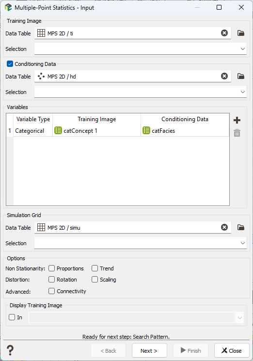
In the Input page, you need to provide:

• Training Image: Select TI
• Conditioning Data: you can indicate that you have some borehole data and want to produce a conditional simulation. For that, you must select the corresponding data table, hd, and then you can add a selection.
• Variables: select the type of variable, which can be categorical or numerical (in this example: categorical)
• Simulation Grid: Select the simu grid

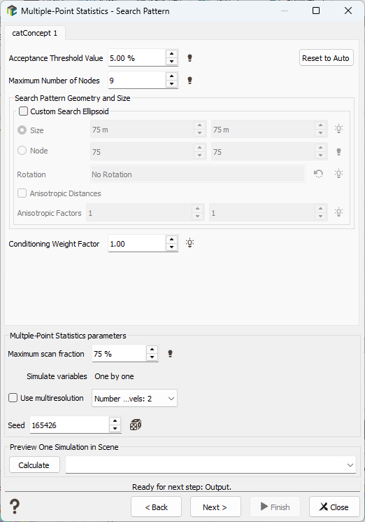
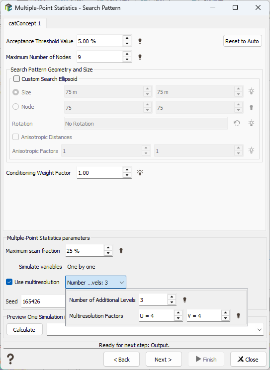
No options are taken into account at the moment, you can click on Next to reach the second page. In the Search Pattern page, several important technical parameters have to be defined:

• Acceptance threshold value (t): The initial value is 5%. Keep it for the moment.
• Search pattern geometry and size: It allows to define the geometry of the search neighborhood ellipsoid and the maximal number of nodes in the patterns. We will keep the default ellipsoid and just set the value of N: the Maximal number of nodes equal to 9.
• Multiple-point statistics parameters: You provide the Maximal scanned fraction (f). Keep the value by default to start (25%).

Note: The three parameters are related to the simulation algorithm, which works in three steps, illustrated in the figure below:

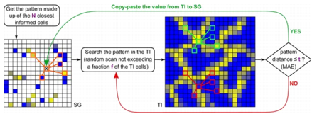
• Step 1: In the output simulation grid, a target point to be simulated is chosen at random. The N closest informed points are then associated to this target point. Informed points correspond to data points and already simulated grid cells. The value N is the “Maximum number of nodes” required by Isatis.neo.
• Step 2: The target point and the N closest informed points define a geometric pattern, centered on the target point with peripheral points corresponding to informed data. This pattern is superimposed to the Training Image, at a random location. Then, the algorithm checks whether the facies configuration in the peripheral points is the same in the TI as in the simulation grid. If it is the case, the facies located at the pattern center in the TI is assigned to the target point in the simulation grid and the target point becomes a new informed point. If it is not the case, a new random location is chosen in the TI and the comparison process is started again.
• This search can be long, and some interruption criteria have been defined to optimize the computation time:
• Stopping criterion #1: It is accepted that the correspondence between the facies configuration in the pattern can be slightly different in the TI than in the simulation grid. The accepted degree of discrepancy is defined by the “Acceptance Threshold value”, which corresponds to the tolerated percentage of error.
• Stopping criterion #2: If there is no sufficient correspondence between TI and simulation grid, another location in the TI of the pattern center is chosen at random. This iterative process can be long, and it can be optimized by stopping it before the whole TI is scanned. The “Maximum scan fraction” corresponds to the percentage of the whole TI that will be scanned for the pattern analysis. When this threshold is reached and if there is still no good correspondence of the pattern facies configuration between TI and simulation grid, the target point in the simulation grid is put at “undefined value” and another target point is chosen at random. Undefined target points are re-analyzed at the end of the simulation, when more informed cells are available.

Maximum scan fraction parameter

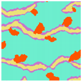
The maximum scan fraction parameter allows you to speed up the simulations but with less accuracy. By raising up to 75% we will gain accuracy.

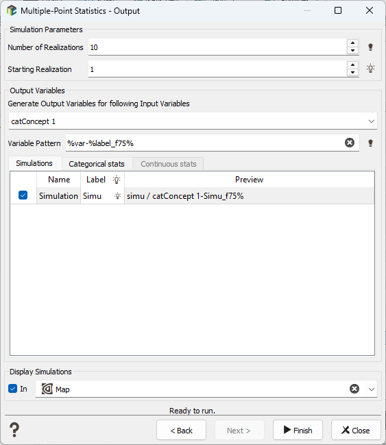
Using the input parameters, set to 75% the maximum scan fraction.

Change the variable pattern (here, %var-%label_f75%) to save the results on other output variables. In this way, we will be able to compare the results.

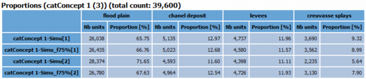
The continuity has been increased compared to the previous simulations.

Be careful that the statistics are almost the same if we compare one by one.

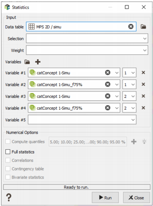
Open the Statistics tool. Select the simulation grid in the data table and the two first indices of each simulation variable to compare the statistics.

Comparison with SIS

The Sequential Indicator Simulations (SIS) allows you to simulate a categorical variable using a sequential indicator method. Here, in order to compare SIS to MPS results, we define parameters to be close to the MPS processing.

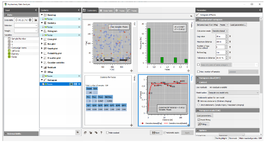
First, using the Exploratory Data Analysis task, we create a Geostatistical set of the Facies variable contained in the hd data table.

Then, we open the SIS task in the Interpolation section.

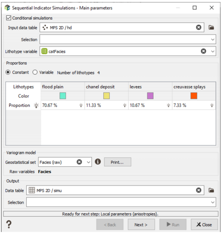
In the first page corresponding to the definition of the input parameters:

• Select the hd data table as conditional data and define the Lithotype variable catFacies.
• The global proportions will be calculated automatically.
• Select the Facies (raw) Geostatistical set created in the previous task.
• Define the simu grid as output data table.

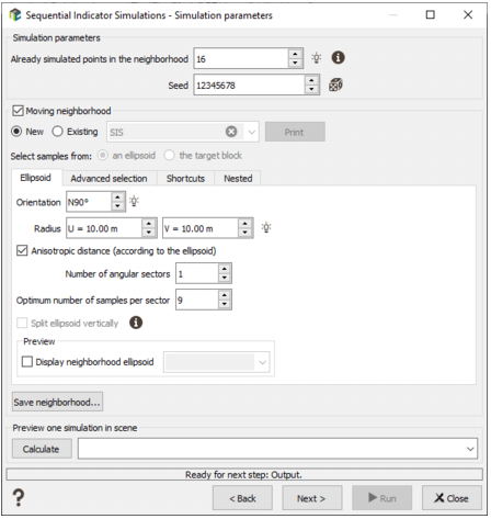
The second page allows the definition of Local anisotropy parameters but it will not be use in our case. The third page is for the neighborhood definition. Select a new moving neighborhood, change the number of sector to 1 and keep the optimum number of samples per sector to 9 (the default value in MPS when working in 2 dimensions).

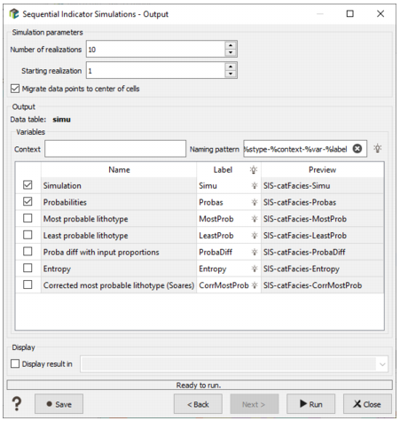
In the last page, we ask for the same number of 10 simulations and check the option Migrate data points to center of cells to ensure the conditional value at the target grid.

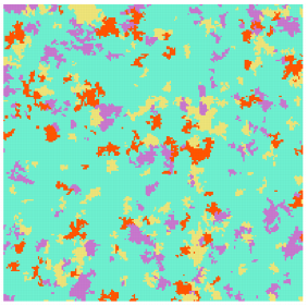
We can see that SIS cannot reproduce the continuity and the pattern of the lithotypes unlike MPS.

MPS using Multi-resolution option

Activate the Multi-Resolution mode which enables to catch multi-scale phenomena more efficiently. When using multi-resolution, the simulations are processed at (N + 1) levels. The first levels (the coarse ones) process large scale patterns, the last levels (the closest to the simulation grid scale) process lower scale patterns.

We perform the simulations:

• Without multi-resolution option,
• With 2 levels of multi-resolution 2x2,
• With 3 levels of multi-resolution 4x4.

The multi-resolution option is set in the search pattern step.

Without multi-resolution option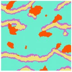
With 2 levels of multi-resolution 2x2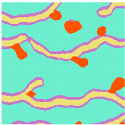
With 3 levels of multi-resolution 4x4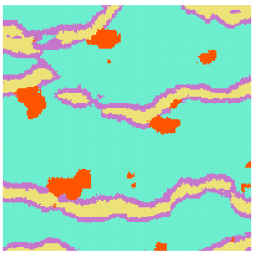

The multi-resolution parameters must be defined wisely, several levels and factors do not mean that the simulations will be accurate.