Preparing and running PGS simulations

• Preparing and running PGS simulations
• • Creating flattened grids
  • Defining lithotypes (conditioning data for PGS)
  • Calculating lithotypes proportions models
  • • Case 1: Global VPC
    • Case 2: 3D estimation of proportions
  • Calculating PGS simulations in flattened grids

Creating flattened grids

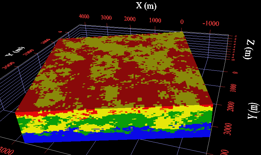
The folded sedimentary layers show a locally varying anisotropy. So, either this anisotropy variation should be modeled or the sedimentary layers should be restored to prior to folding. Flattening the sedimentary layers could be done by the function of "Unfolding and Unfaulting" accessible through Interpolation / Processing. There are three options for unfolding:

1. Parallel to the Top or to the Base of the stratigraphic unit;
2. parallel to a user defined Unfolding Model (Reference Marker), which can be inside or outside the stratigraphic unit (a maximum flooding surface, typically);
3. proportional between Top and Base.

The unfolding parallel to a horizon is:

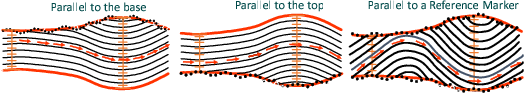
The proportional unfolding is illustrated below. Several options can be considered, according to the orientation of the pillars along which the distance between Top and Base is calculated. In the simplest case, pillars are vertical. In the standard case, pillars are perpendicular to a surface, which can be the top, the base or an intermediate surface as shown on the right side:

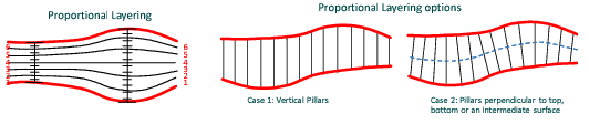
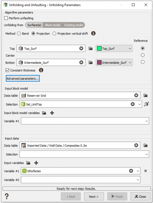
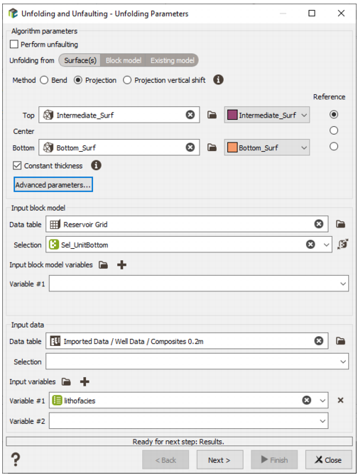
In this tutorial, we will select a proportional unfolding in the standard case, the reference horizon for defining pillars orientation being an intermediate surface in the middle of the interval between top and bottom of each stratigraphic unit. The parameters to be selected for using this option are:

• Projection method,
• Top_Surf as the Top surface and the Reference,
• Intermediate_Surf as the Bottom,
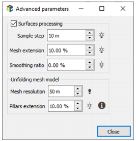
• In the Advanced parameters, check the Surfaces processing toggle. Set a Mesh resolution of 50m instead of 20m to speed up the calculations and regarding the triangle size of the surfaces.
• Select the Reservoir Grid as the Data table of the Input block model with the Sel_UnitTop Selection.
• Select the Composites 0.2m of the Well Data as the Data table of the Input data with the lithofacies variable.

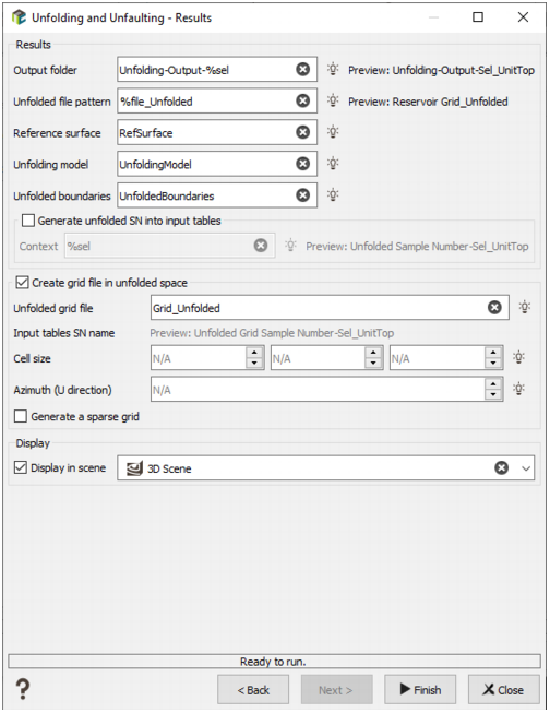
The output unfolded grid name is defined in the second window. Take note that it is recommended to activate the Generate a sparse grid option, a sparse grid being much less demanding in disk space. For this tutorial, as the percentage of empty cells in the complete original grid is low, we can deactivate it.

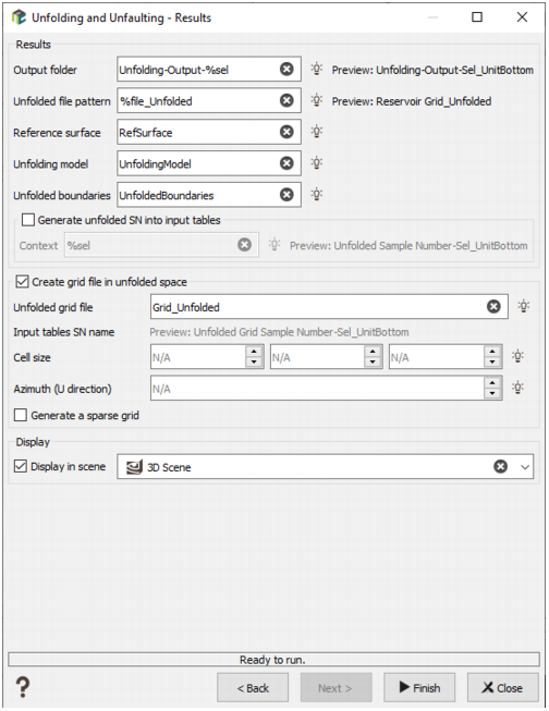
The unfolding operation must be repeated for the lower stratigraphic unit. The options to be considered are:

Defining lithotypes (conditioning data for PGS)

The lithofacies input variable is made of many rock categories. It will be transformed into the lithotype variable to be simulated. Lithotypes correspond to groups of lithofacies related to the same depositional environment. This operation is meant to reduce the number of categories to be simulated (compared to the large amount the lithofacies). Lithotypes are defined according to the geologist knowledge, and Isatis.neo allows defining several sets of lithotypes, corresponding to different groups of lithofacies, to test different sedimentological interpretations. This transformation may simply be skipped if the lithofacies already refers to the lithotype data.

In this example, we define 4 lithotypes per stratigraphic unit, whose definition and attributes will be provided in the dedicated panels.

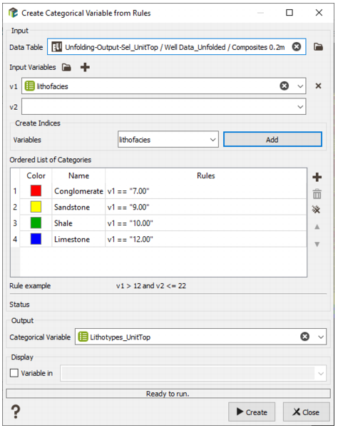
The lithotypes definition is made by creating a specific categorical variable in each lithostratigraphic unit, using the menu item “Data management / Create / Create Categories / From Rules”. In Isatis.neo, when a categorical variable is created from rules, an input variable must be defined and categories are defined by applying rules on this input variable. In our case, the input variable is “lithofacies” and the rules define how the lithofacies are merged in each stratigraphic unit. The results are stored in an output variable. Note that defining different output variables corresponding to different rules allow testing different sedimentological interpretations.

Merging Rules and color scale to be applied are illustrated below. It can be noticed that the lithotypes correspond to different lithofacies in the two lithostratigraphic units.

Note: To assign a color to a category, just click on the corresponding colored square in the list of categories.

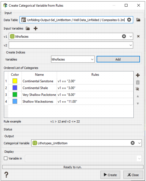
Choosing different lithofacies merging rules in different lithostratigraphic units has a practical consequence. If a lithofacies selected in a lithotype from the first lithostraphic unit appears in a second lithostratigraphic unit where it is not selected in a lithotype, then an undefined value is assigned to the corresponding sample in the second lithostratigraphic unit. This configuration occurs in very few samples near the contact between the upper and lower lithostratigraphic units, due to discretization effects. If the number of undefined samples in a given lithostratic unit is high, it may indicate a mapping issue with at least one of the limiting horizons or with the reference horizon for flattening. In this Case Study, this event is so rare that it has no impact and the approximation consisting in assigning an undefined value to these samples is acceptable.

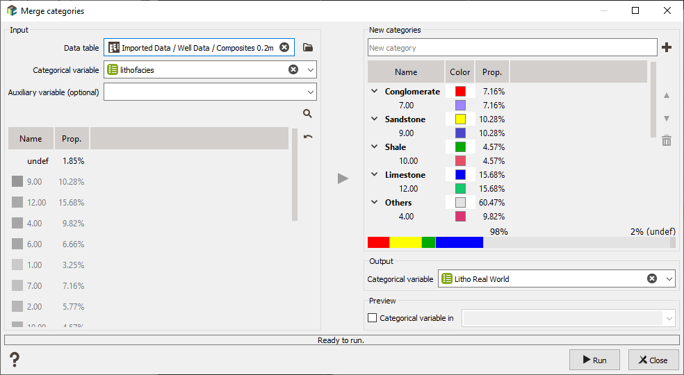
The same lithotype variable can be created on the composite samples. An alternative to the Create Categorical Variable from Rules task consists in using the menu item “Data management / Create / Create Categories / Merge Categories”. It allows you to easily create a new categorical variable (with a new catalog) from another one by selecting the input categories and grouping some of them into new categories.

Calculating lithotypes proportions models

The lithotypes proportions in working (flattened) grids are an essential ingredient of the plurigaussian model. They correspond to the numerical equivalent of the sedimentological conceptual interpretation and are an important soft constraint in many categorical variables simulation methods. Therefore, they must be calculated carefully, in each lithostratigraphic unit.

This operation is made with the menu item “Interpolation / Processing / Proportion Modeling”.

Isatis.neo offers several techniques for calculating the lithotypes proportion model:

• Global Vertical Proportion Curve (VPC) calculation;
• Proportion estimation in 3D, from well data, using a specific algorithm based on Stochastic Partial Differential Equations (SPDE) interpolation approach;
• Proportion estimation as in the previous case, with an additional constraint made of a 2D map of a variable correlated with the average proportion in the studied lithostratigraphic unit.

In this Case Study, two options will be considered:

1. A first calculation with a global VPC, which assumes that we are in the stationary case
2. A second calculation with an estimated 3D model of proportions, which will allow lateral variations of facies (non-stationary case).

Case 1: Global VPC

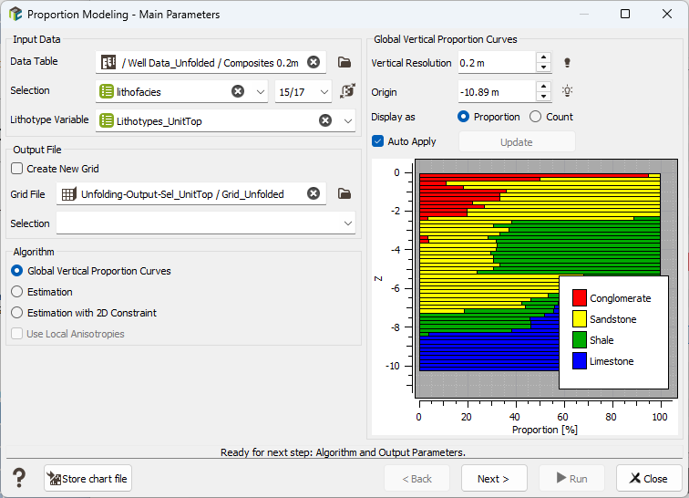
A Vertical Proportion Curve (VPC) is a stacked bar diagram that represents the vertical evolution of the proportion of each lithotype. Each line of the graph represents a layer in the simulation grid (flattened), calculated from discretized well data. VPCs are used to interpret the vertical variability of the lithotypes in a deposit. This tool is very useful for the geologist as it gives an idea of the original (before deformation) distribution of the lithotypes. The lithostratigraphy can be studied to understand the deposit genesis.

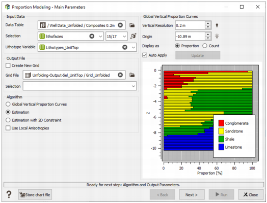
A VPC example is illustrated here with its input parameters, the option “Global Vertical Proportion Curve” being selected. This figure represents the first window of the Proportion Modeling workflow.

In this first case, the VPC is used for calculating the lithotypes proportions in any cell of the simulation grid.

A selection must be defined to exclude samples where the initial lithofacies is not defined. Select the lithofacies variable as categorical selection and uncheck the category "0" to exclude the value from the calculation.

It can be noticed that the proportions can be stored in the simulation grid (which is the proposed option) or in another grid if the check box “Create New Grid” is checked. In such a case, proportions are stored in a grid which is geometrically consistent with the simulation grid, but which can be coarser.

Click on the button “Next” to go to the second window of the workflow, to define the smoothing parameter and the output variable.

The calculation of a VPC from wells may lead to a noisy graph. The result can be regularized by making a vertical moving average of proportions. In Isatis.neo, the proportion at a given layer is averaged with the proportions in the layer above and in the layer below. The smoothing parameter defines how many times this moving average is repeated. The higher is this number, the smoother is the result.

The required output is a macro-variable in which the proportions of each lithotype will be stored. This variable is defined in each cell of the simulation grid.

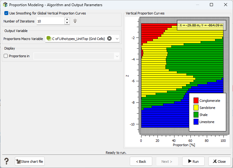
An example of the proportion model for sandstone:

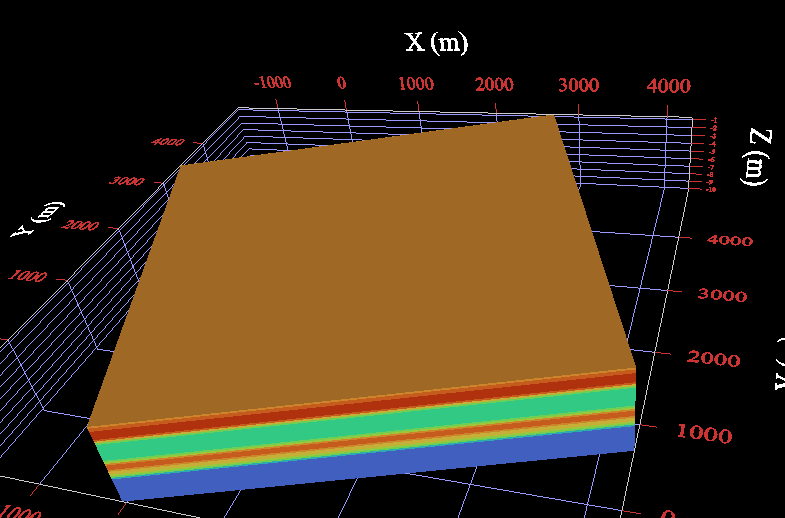
As we used a global VPC, the proportion of a given lithotype is constant in a given layer, which leads to the stratified look of the proportions model.

Case 2: 3D estimation of proportions

In this second case, the proportion model results from a 3D estimation from well data. The algorithm is based on the Stochastic Partial Differential Equations framework, in which estimations lead to similar results as kriging.

The first window of the “Proportions Modeling” workflow is the same as in the previous case, but this time the “Estimation” algorithm is selected.

Click Next to go to the second window of the workflow.

A slider allows you to adjust the algorithm technical main parameters (The higher is this precision, which means the closest to 1, the smoother and the more spatially continuous are the output proportions). A button gives access to some advanced parameters. Please refer to the technical documentation for details.

In this Case Study, consider first the default parameters:

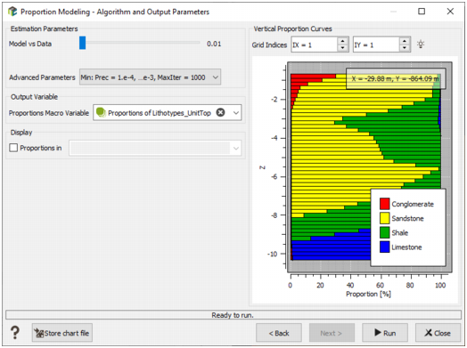
An example of the proportion model for sandstone is illustrated here. This time, the proportion model is varying in space within each layer.

Calculating PGS simulations in flattened grids

The Pluri-Gaussian simulation process consists in simulating lithotypes by thresholding two continuous Gaussian simulations. It is performed in 4 steps:

1. Conditional simulations of the 2 underlying Gaussian random fields at the data point using a Gibbs Sampler algorithm. It allows assigning Gaussian values at data points which will provide the right lithotype after thresholding.
2. Non-conditional simulations of the 2 Gaussian random fields at each node of the Working Grid (the flattened grids in this Case Study).
3. Conditioning of the 2 previous Gaussian simulations, using the results of step 1 as conditioning data.
4. Thresholding of the two Gaussian simulations to get the simulated lithotypes. The thresholds are calculated from the Lithotype proportion model and the Lithotype rules.

This implementation of the Pluri-Gaussian Simulation methodology is innovative and different than the usual implementations. Traditionally, the variograms of the two underlying Gaussian random functions are inferred from the experimental variograms of the lithotypes indicator functions. Here, we calculate directly the variograms of the Gaussian values assigned to each sample where a lithotype is defined. Details about this methodology can be found in:

Nicolas Desassis, Didier Renard, Hélène Beucher, Sylvain Petiteau, Xavier Freulon. A pairwise likelihood approach for the empirical estimation of the underlying variograms in the plurigaussian models. 2015. hal-01213962v2.

At this stage of the Case Study, the flattened working grid with discretized data and the Lithotype proportion model are already available. The Lithotype rules and the variograms of the two Gaussian random fields are not yet available and must be defined and inferred from data.

This is the purpose of the Pluri-Gaussian Simulations workflow, which can be accessed from the menu item “Interpolation / Risk Analysis / Plurigaussian simulations”.

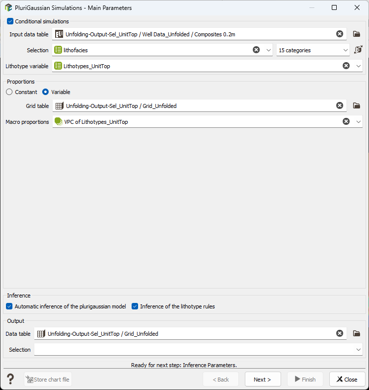
The workflow is made of six windows, the first one being dedicated to the definition of input data and lithotypes. This first window is shown in the following snapshot, with the input data corresponding to the Case 1 previously defined (global VPC).

It can be noticed that you have the choice of using automatic inference procedures for the variograms model and the Lithotype rules, or to make these inferences manually. For that, you simply have to uncheck the checkboxes ”Automatic inference of the Plurigaussian model” and “Inference of the Lithotype rules”. Please refer to the Isatis.neo User Guide for details.

For this Case Study, start by keeping automatic inference options activated and the default experimental variogram parameters.

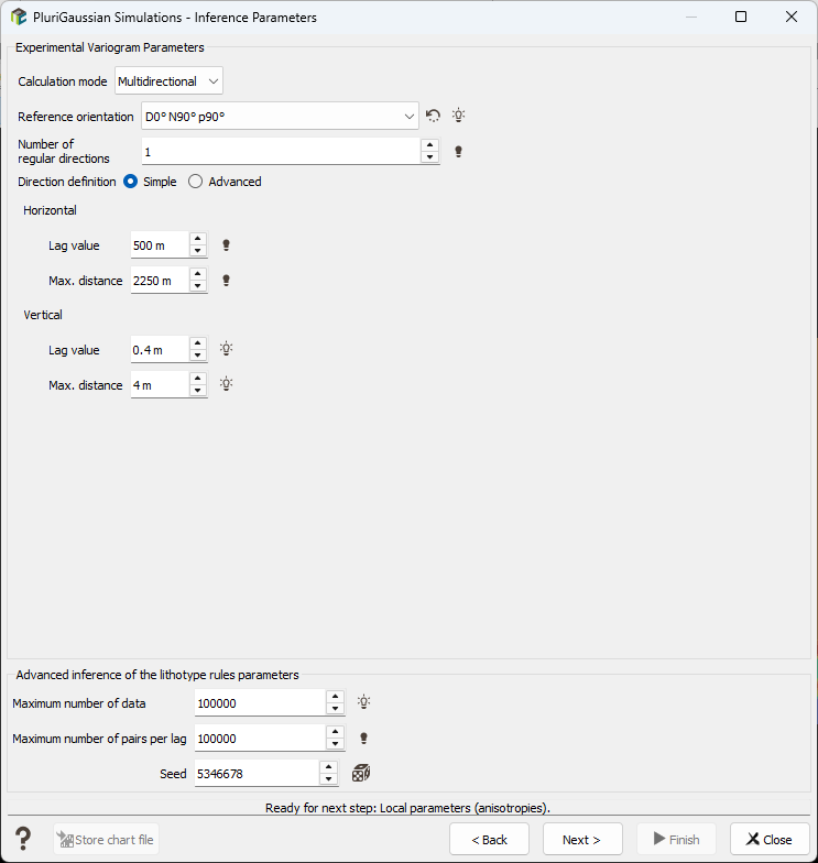
Click on the button “Next” to go to the second window of the workflow.

The second window is dedicated to the experimental variogram parameters of the Lithotype variable. Define only 1 regular direction with a lag value of 500m and a maximum distance of 2250m in the horizontal direction. Leave the other parameters to automatic for the vertical direction.

One the third and fourth windows, specifications of local anisotropy and neighborhood parameters may be precised, which remains empty for the current case-study. The fifth window of the Pluri-Gaussian workflow is dedicated to the variogram model fitting and to the definition of the Lithotype rules.

The window which is displayed below corresponds to the automatic inference of variograms and rules.

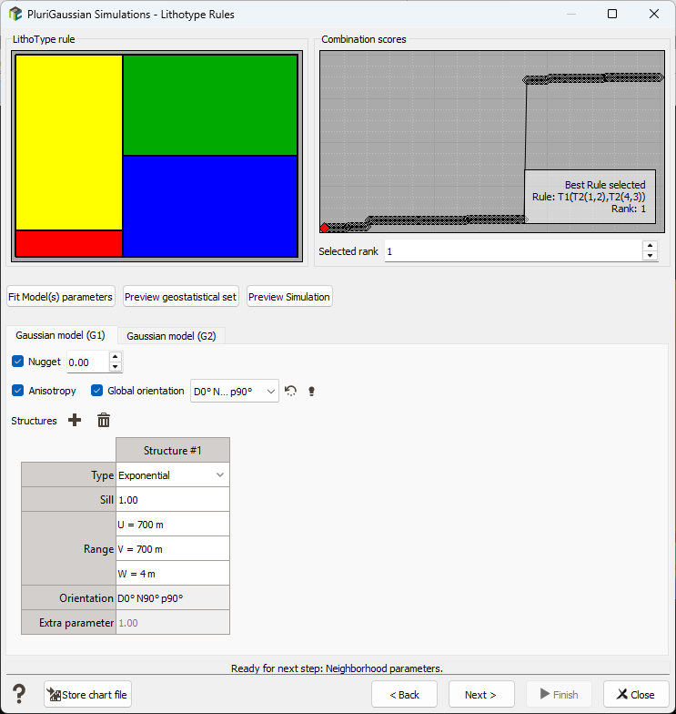
At the top of the window, the Lithotype rule (also known as ’flag’) is displayed on the left and the Combinaison score graphic is on the right. Each point of this graph corresponds to an evaluated Lithotype rule. All the Lithotype rules that can be defined with the selected number of lithotypes are tested for fitting the variogram models, which depend on these rules. The maximal likelihood, regarding the experimental curves, is evaluated and the Lithotype rules are ordered according to the performance criterion of the fitting. Then, the Combinaison score graph is built, the points being ordered from the "best" one (lowest score on the left) to the "worst" one (highest scores on the right). The displayed Lithotype rules is the one with best score.

If you prefer to choose another rule, you can click on the different points of the ranking graph to display another possibility. The one which is displayed when going to the next step is automatically selected.

Take note that it is not recommended to define more than six lithotypes, due to the exponential increase of lithotype combinations, which severely penalizes the Lithotype rules ranking algorithm.

The automatically fitted variogram models for the two underlying Gaussian random functions are displayed on the bottom part of the window. These models can be edited manually. By clicking on the button “Preview Simulation”, you can display a non-conditional simulation calculated with the selected Lithotype rule and Variograms. Details can be found in the Isatis.neo User Guide.

For this Case Study, start by selecting the default models and rules.

Click on the button “Next” to go to the last window of the workflow, which is dedicated to the simulations context and output parameters definition:

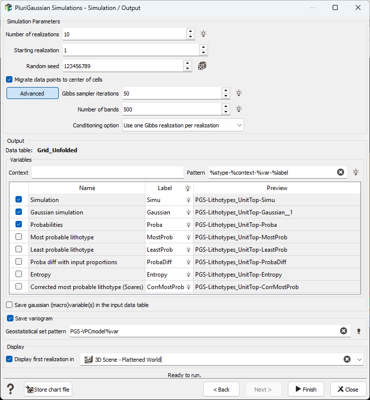
You can choose the number of simulations to be calculated. A set of 10 realizations is proposed, but you can increase this number, the calculations being quite fast in this simple Case Study which is using small grids.

The random seed can also be edited. This parameter is important, as it allows reproducing the same simulations later if they have not been stored. Calculations made at different dates with the same input parameters (variograms and Lithotype rules, conditioning data, proportions model) and the same seed will provide exactly the same results. With the same input parameters and different seeds, the results will have the same statistical characteristics but will be different.

When the number of simulations is more than 1, the random seed is automatically updated at each iteration (10 is added to the previous seed).

The starting realization number can be modified. It allows calculating a high number of simulations in several steps. You can for example calculate first 10 simulations with a given initial random seed. If you calculate 10 additional simulations later, by starting at the realization 11, with the same initial random seed, then you will get the same results as if you had calculated 20 simulations at the first time.

The "Migrate data points to center of cells" option ensures the consistency of the simulations by migrating the input data points prior to conditioning the simulations. We check the option in our case.

Click on the Advanced button to access to additional parameters and change the Conditioning option to Use one Gibbs realization per realization. This method is slower if you have an important amount of input samples but it introduces more variability.

In the end, you can store in the output (flattened) grid the Lithotype simulations (macro-variable with the selected number of realizations), the Gaussian simulations before thresholding (2 macro-variables with the selected number of realizations) and the Lithotype proportions calculated from all the realizations (macro-variable with the number of lithotypes). Other post-processing results can be calculated (most and least probable facies, probability differences with input proportions, entropy map and most probable facies corrected through the Soares method) but they are not stored in this example.

The process can be repeated with the estimated 3D model of proportions. You will simply have to update the name of the variable which contains the proportions model in the first window and possibly adjust the Lithotype rules and variograms (or keep the automatic fitting results).

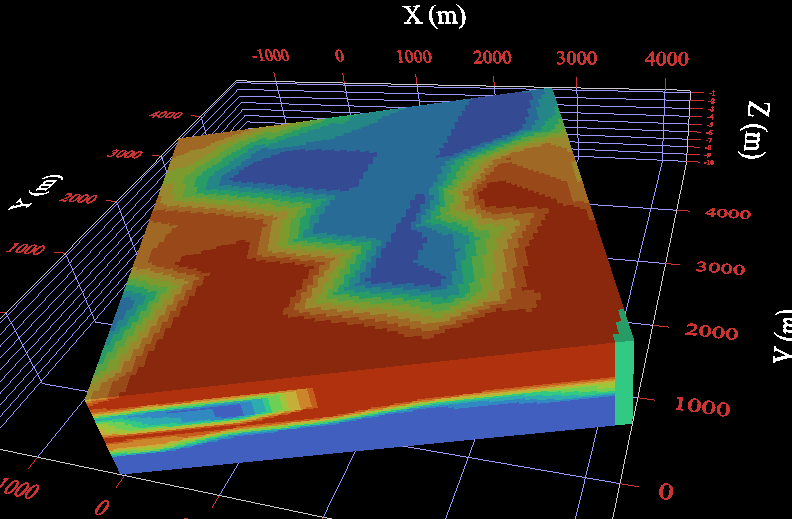
An example of Pluri-Gaussian simulation results for the upper lithostratigraphic unit is illustrated below. It corresponds to the case where a 3D model of lithotypes proportion is used.