Presentation of the dataset
Creation of a new project
First, before loading the data, create a new project using the Project Manager functionality presented below.
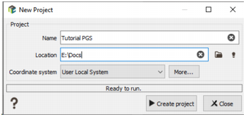
You can see that the coordinate system can be defined by the user. At the creation of a new Isatis.neo project, you need to select a coordinate system that will be used to unify your data. For this case study, we choose the User Local System.
Note: A link to all the EPSG codes on the official site of Spatial Reference is also provided http://www.spatialreference.org/ref/epsg/. In this site, you can find other codes like the Proj4 code for example.
If a coordinate system has been defined for a project, the imported data will be automatically converted to the defined coordinate system of the project.
In this case study, as the User Local System has been selected, any new data must be consistent with this local system of coordination. It is the user’s responsibility to ensure the consistency of the imported data of different sources, for example topography, well tops, etc.
Creation of a new folder in Isatis.neo database
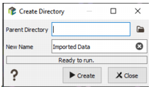
The imported data will be stored in a dedicated new folder. This folder can be created as follows:
In the empty data explorer, click on the right mouse button to display a contextual menu allowing to create a new folder in the database. Select this option.
A window is displayed, in which you can define the name of the new folder. Let the Parent Directory empty:
Data Loading and Visualization
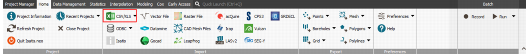
The formatted data can be loaded using the wizard which can be accessed from Home/Import/Excel/Wells:
The wizard is made of four successive windows:
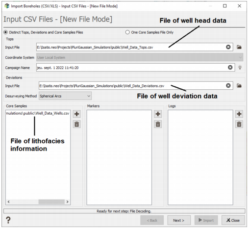
On the first window, you are asked to create a new data file in Isatis.neo or to add information to an existing data file. Select the first option New File by clicking on it.
It automatically opens a window from which you can load the three Excel files with well data: Well_Data_Tops.csv, Well_Data_Deviations.csv and Wells_Data_Wells.csv. These files are located in the Isatis.neo installation directory/Datasets/PluriGaussian Simulations or in the public directory of your project if this one has been restored). Enter the file names in the corresponding text fields, and click on the Next button.
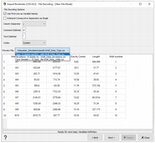
The next window allows you to check your data. You can check the different files by selecting them from a list. If everything looks fine, click on the Next button.
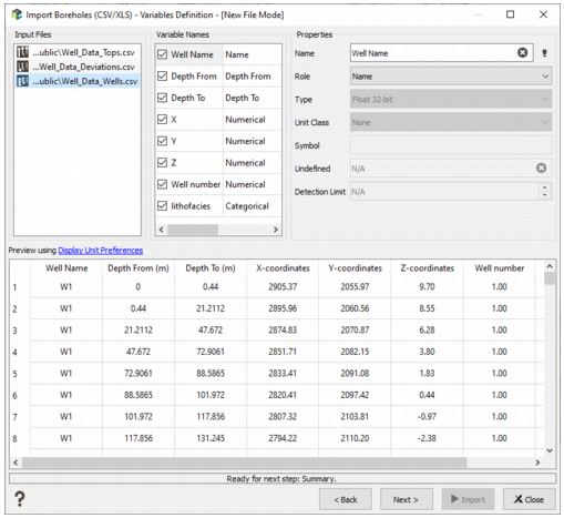
The third window allows you editing the data. At this stage, you can update the variables name or unit. When edition is completed, click on the Next button.
The last window provides a summary of data to be imported and asks you for a data file name in Isatis.neo. This name corresponds to file and directory names in the data hierarchic organization.
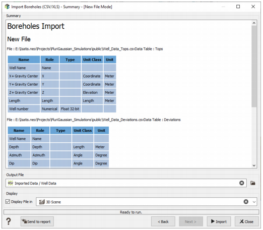
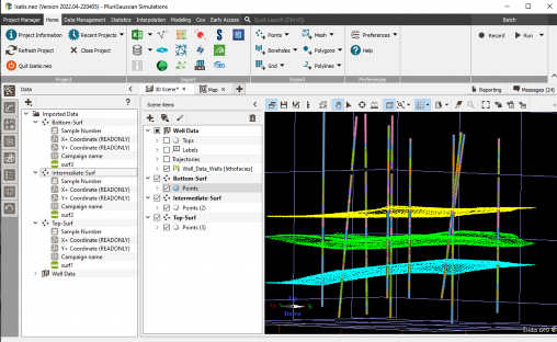
Click on the Import button to load the well data. They will appear in the Isatis.neo data tree, and in the scene if the Display option is active.
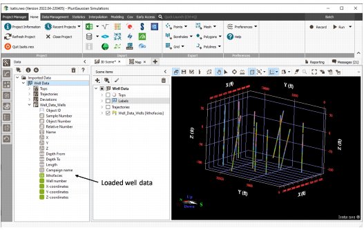
Note: The wells are not very deep, and many of them have a very shallow dip. A vertical exaggeration of 50 is applied in the previous scene ("Z scale" parameter located in the 3D scene toolbar).
Horizons data loading and visualization
The file surf1.csv corresponds to the top of the upper stratigraphic unit, the file surf2.csv corresponds to the contact between the upper and lower stratigraphic units, and the file surf3.csv represents the base of the lower stratigraphic unit. These surfaces are punctual data.
Load first the top surface surf1.csv.
The formatted data can be loaded using the wizard accessible through the menu item Home/Import/Excel/Points.
The wizard is made of 4 successive windows:
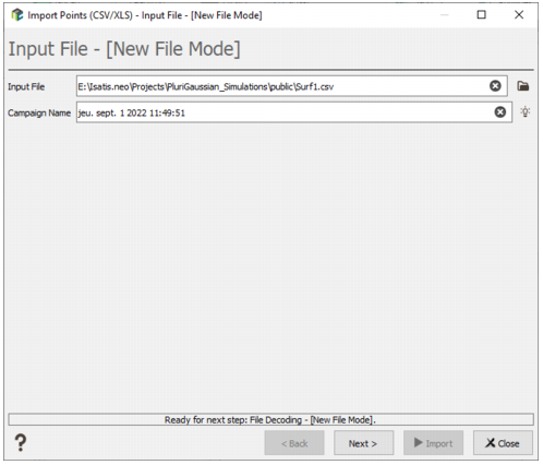
The first one asks you to create a new data file in Isatis.neo or to append the imported information to an existing data file. Select the first option “New File” by clicking on it. So a window will be opened, asking for the Excel file with surface data to be loaded. Enter the file name in the corresponding text field and click on the button “Next”.
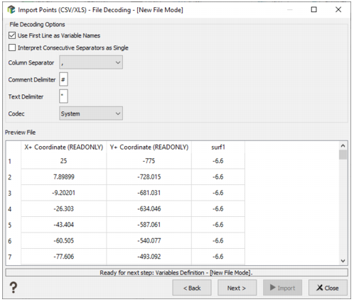
The next window allows you to check your data. You can check the different files by selecting them from a list. If everything looks fine, click on the Next button.
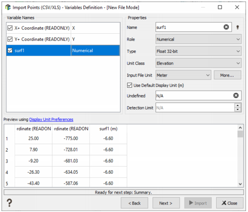
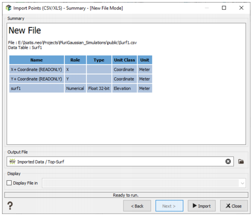
The third window allows you editing the data. At this stage, you can update the variables name or unit. Be careful that the surf1 variable is defined as a Numerical variable (and not Z), otherwise your data will be 3D and not 2D. You can set its Unit Class to Elevation in Meter. When edition is completed, click on the Next button.
The last window provides a summary of data to be imported and asks you for a data file name in Isatis.neo. This name corresponds to a directory name in the data hierarchic organization.
The same operation must be repeated for the two other surfaces.
In the end, you should get the following data: