The Experimental Variability Functions

• The Experimental Variability Functions
• • Univariate case
  • Weighted Variability Functions
  • Multivariate case
  • Variogram Transformations

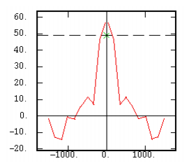
Though the variogram is the classical tool to measure the variability of a variable as a function of the distance, several other two-points statistics exist. Let us review them through their equation and their graph on a given data set. n designates the number of pairs of data separated by the considered distance and Z_α and Z_β stand for the value of the variable at two data points constituting a pair.

• is the mean over the whole data set
• is the variance over the whole data set
• is the mean calculated over the first points of the pairs (head)
• is the mean calculated over the second points of the pairs (tail)
• is the standard deviation calculated over the head points
• is the standard deviation calculated over the tail points
• α and β. β is considered to be at a distance of +h from α.

Univariate case

The Transitive Covariogram
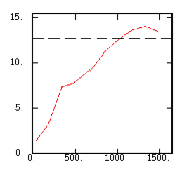
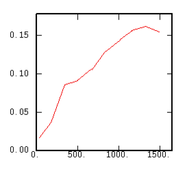
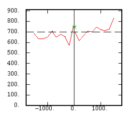
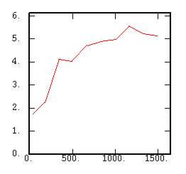
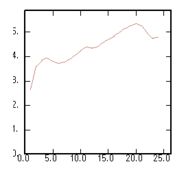
The Variogram
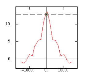
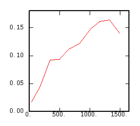
The Covariance (centered)
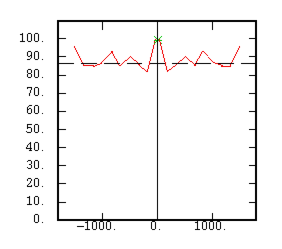
The Non-Centered Covariance
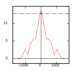
The Non-Ergodic Covariance
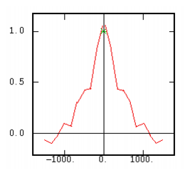
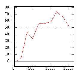
The Correlogram
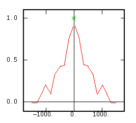
The Non-Ergodic Correlogram
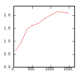
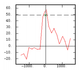
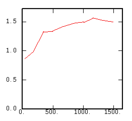
The Madogram (First Order Variogram)
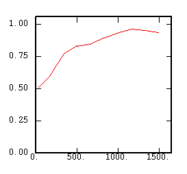
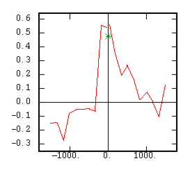
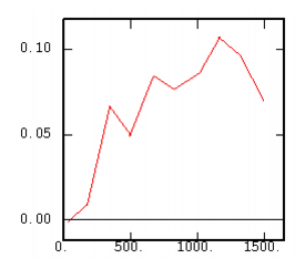
The Rodogram (1/2 Order Variogram)
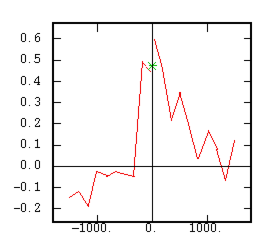
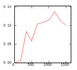
The Relative Variogram
The Non-Ergodic Relative Variogram
The Pairwise Relative Variogram

Although the interest of the madogram and rodogram, as compared to the variogram, is quite obvious (at least graphically), as it tends to smooth out the function, the user must always keep in mind that the only tool that corresponds to the statement of kriging (namely minimizing a variance) is the variogram. This is particularly obvious when looking at the variability values (measured along the vertical axis) on the different figures, remembering that the experimental variance of the data is represented as a dashed line on the variogram picture.

Weighted Variability Functions

It can be of interest to take into account weights during the computation of variability functions. These weights can for instance be derived from declustering; in this case, their integration is expected to compensate potential bias in the estimation of the experimental function from clustered data. For further information about these weighted variograms, see for instance Rivoirard J. (2000), Weighted Variograms, In Geostats 2000, W. Kleingeld and D. Krige (eds), Vol. 1, pp. 145-155.

For instance, the weights are integrated in the weighted experimental variogram equation in the following way:

The other experimental functions are obtained in a similar way.

Multivariate case

In the multivariate case kriging requires a multivariate model. The variograms of each variable are usually designated as "simple" when the variograms between two variables are called cross-variograms.

We will now describe, through their equation, the extension given to the statistical tools listed in the previous section, for the multivariate case. We will designate the first variable by (Z) and the second by (Y), and and refer to their respective means over the whole field, and to their means for the head points, and to their means for the tail points.

The Transitive Cross-Covariogram
The Cross-Variogram
The Cross-Covariance (centered)
The Non-Centered Cross-Covariance
The Non-Ergodic Cross-Covariance
The Cross-Correlogram
The Non-Ergodic Cross-Correlogram
The Cross-Madogram
The Cross-Rodogram
The Relative Cross-Variogram
The Non-Ergodic Relative Cross-Variogram
The Pairwise Relative Cross-Variogram
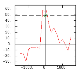
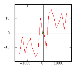
This time most of the curves are no longer symmetrical. In the case of the covariance, it is even convenient to split it into its odd and even parts as represented below. If designates the distance (vector) between the two data points constituting a pair, we then consider:
The Even Part of the Covariance
The Odd Part of the Covariance

A last remark concerns the presence of information on all variables at the same data points: this property is known as isotopy. The opposite case is heterotopy: one variable (at least) is not defined at all the data points.

The kriging procedure in the multivariate case can cope nicely with the heterotopic case. Nevertheless, in the meantime one has to calculate cross-variograms which can obviously be established from the common information only. This consideration is damaging in a strong heterotopic case where the structure, only inferred on a small part of the information, is used for a procedure which possibly operates on the whole data set.

Variogram Transformations

Several transformations based on variogram calculations (in the generic sense) are also provided:

The ratio between the cross-variogram and one of the simple variograms:		When this ratio is constant, the variable corresponding to the simple variogram is "self-krigeable". This means that in the isotopic case (both variables measured at the same locations) the kriging of this variable is equal to its cokriging. This property can be extended to more than 2 variables: the ratio should be considered for any pair of variables which includes the self-krigeable variable.
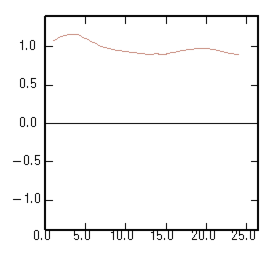
The ratio between the square root of the variogram and the madogram:		This ratio is constant and equal to for a standard normal variable, when its pairs satisfy the hypothesis of binormality. A similar result is obtained in the case of a bigamma hypothesis.
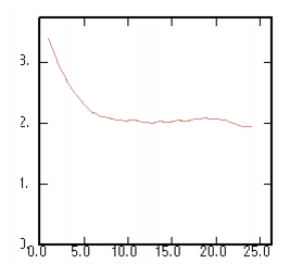
The ratio between the variogram and the madogram:		If the data obeys a mosaic model with tiles identically and independently valuated, this ratio is constant.
The ratio between the cross-variogram and the square root of the product of the two simple variograms:	When two variables are in intrinsic correlation, the two simple variograms and the cross variogram are proportional to the same basic variogram. This means that this ratio, in the case of intrinsic correlation must be constant. When two variables are in intrinsic correlation cokriging and kriging are equivalent in the isotopic case.