Variogram Model
Basic Structures
The following pages illustrate all the basic structures available in Isatis to fit a variogram model on an experimental variogram. Each basic structure is described by:
- its name.
-
its mathematical expression, which involves:
- A coefficient which gives the order of magnitude of the variability along the vertical axis (homogenous to the variance). In the case of bounded functions (covariances), this value is simply the level of the plateau reached and is called the sill. The same concept has been kept even for the non-bounded functions and we continue to call it sill for convenience. The interest of this value is that it always comes as a multiplicative coefficient and therefore can be calculated using automatic procedures, as explained further. The sill is equal to "C" in the following models.
-
A parameter which affects the horizontal axis by normalizing the distances: hence the name of scale factor. This term avoids having to normalize the space where the variable is defined beforehand (for example when data are given in microns whereas the field extends on several kilometers). This scale factor is also linked to the physical parameter of the selected basic function.
When the function is bounded, it reaches a constant level (sill) or even changes its expression after a given distance: this distance value is the range (or correlation distance in statistical language) and is equal to the scale factor. For the bounded functions where the sill is reached asymptotically, the scale factor corresponds to the distance where the function reaches 95% of the sill (also called practical range). For functions where the sill is reached asymptotically in a sinusoidal way (hole-effect variogram), the scale factor is the distance from which the variation of the function does not exceed 5% around the sill value.
This is why, in the variogram formulae, we systematically introduce the coefficient ẟ (norm) which gives the relationship between the Scale Factor (SF) and the parameter a:
.
For homogeneity of the notations, the ẟ norm and a are kept even for the functions which depend on a single parameter (linear variogram for example): the only interest is to manipulate distances "standardized" by the scaling factor and therefore to reduce the risk of numerical instabilities.
Finally, the scale factor is used in case of anisotropy. For bounded functions, it is easy to say that the variable is anisotropic if the range varies with the direction. This concept is generalized to any basic function using the scale factor which depends on the direction, in the calculation of the distance.
- A third parameter required by some particular basic structures α.
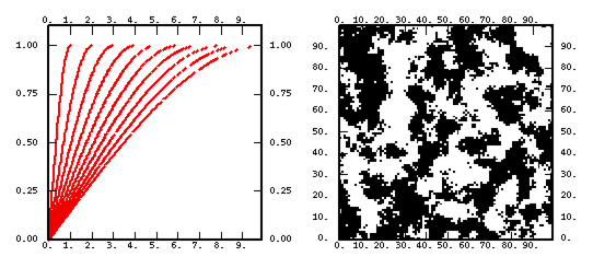
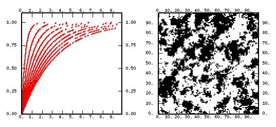
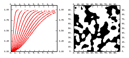
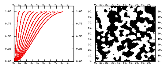
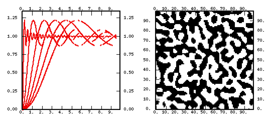
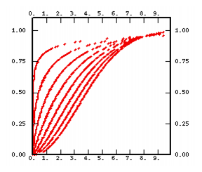
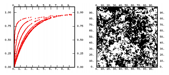
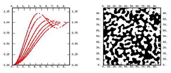
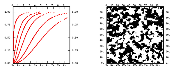
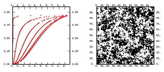
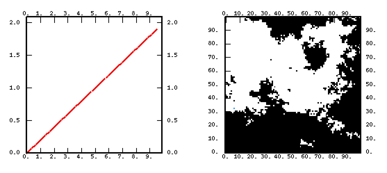
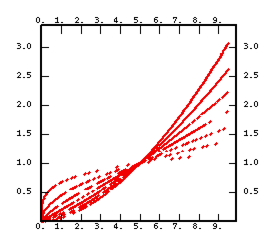
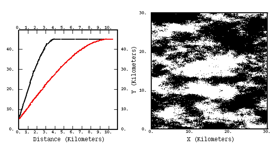
- a chart representing the shape of the function for various values of the parameters.
- a non-conditional simulation performed on a 100 X 100 grid. As this technique systematically leads to a normal outcome (hence symmetrical), we have painted positive values in black and negative ones in white. Except for the linear model where the median is used as a threshold.
The Anisotropy
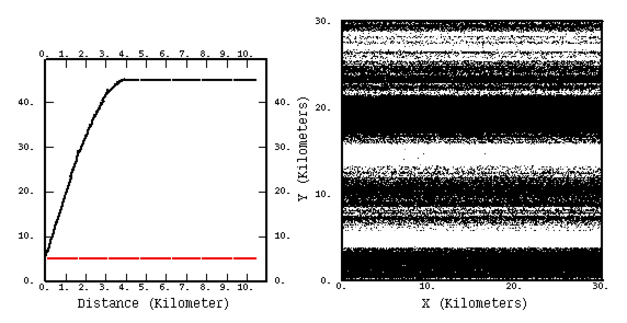
By anisotropy we mean the difference in the variability of the phenomenon in the different directions of the space. For the practical description (in 2D) of this concept, we focus on two orthogonal directions and distinguish between the two following behaviors, illustrated through basic structures with sill and range:
-
same sill, different ranges: geometric anisotropy
Its name comes from the fact that by stretching the space in one direction by a convenient factor we also stretch the corresponding directional range until it reaches the range on the orthogonal direction. In this new space, the phenomenon is then isotropic: the correction is of a geometric nature.
-
same range, different sills: zonal anisotropy
This describes a phenomenon where its variability is larger in one direction than in the orthogonal one. This is typically the case for vertical orientation through a "layer cake" deposit by opposition to any horizontal orientation. No geometric correction will reduce this dissimilarity
-
Practical calculations
The anisotropy consists of a rotation and the ranges along the different axes of the rotated system. The rotation can be defined either globally or for each basic structure.
In the 2D case, for one basic structure, and if "u" and "v" designate the two components of the distance vector in the rotated system, we first calculate the equivalent distance:
where au and av are the ranges of the model along the two rotated axes.
Then this distance is used directly in the isotropic variogram expression where the range is normalized to 1.
In the case of geometric anisotropy, the value au/av corresponds to the ratio between the two main axes of the anisotropy ellipse.
For zonal anisotropy, we can consider that the contribution of the distance component along one of the rotated axes is discarded: this is obtained by setting the corresponding range to "infinity".
Obviously, in nature, both anisotropies can be present, and, moreover, simultaneously.
Finally the setup of any anisotropy requires the definition of a system: this is the system carrying the anisotropy ellipsoid in case of geometric (or elliptic) anisotropy, or the system carrying the direction or plane of zonal anisotropy.
This new system is defined by one rotation angle in 2D, or by 3 angles (dip, azimuth and plunge) in 3D. It is possible to attach the anisotropy rotation system globally or individually to each one of the nested basic structures. This possibility leads to an enormous variety of different textures.
Integral Ranges
The integral range is the value of the following integral (only defined for bounded covariances):
A is a function of the dimension of the space. The following table gives the integral ranges of the main basic structures when the sill C is set to 1. with and the parameter α.
| 1-D | 2-D | 3-D | |
|---|---|---|---|
| Nugget Effect | 0 | 0 | 0 |
| Exponential |
|
|
|
| Spherical |
|
|
|
| Gaussian |
|
|
|
| Cardinal Sine |
|
|
|
| Stable |
|
|
|
| Gamma |
|
|
|
| J-Bessel |
|
|
|
| K-Bessel |
|
|
|
| Gen. Cauchy |
|
|
|
Convolution
If we know that the measured variable Z is the result of a convolution p applied on the underlying variable
We can demonstrate that the variogram of Z can be deduced from the variogram of Y as follows:
Therefore, if the convolution function is fully determined (its type and the corresponding parameters), specifying a model for Y will lead to the corresponding model for Z.
Incrementation
In order to introduce the concept of incrementation, we must recall the link between the variogram and the covariance:
where γ(h) is calculated as the variance of the smallest possible increment:
We can then introduce the generalized variogram Γ(h) as the variance of the increment of order (k+1):
where
which requires data to be located along a regular.
The scaling factor Mk is there to ensure that in the case of a pure nugget effect:
The benefit of the incrementation is that the generalized variogram can be derived using the generalized covariance:
Then, we make explicit the relationships between and for several orders :
| k |
|
|---|---|
| 0 |
|
| 1 |
|
| 2 |
|
Generally speaking, we can say that the shape of Γ(h) is not modified when considering K(h):
- if K(h) is a standard covariance (range a and sill C), Γ(h) reaches the same sill C for the same range: its shape is slightly different.
- if K(h) is a generalized covariance of the |h|α type, then Γ(h) is of the same type: the only difference comes from its coefficient which is multiplied by:
Multivariate Case
When several variables are considered simultaneously, we work in the scope of the Linear Model of Coregionalization which corresponds to a rather crude hypothesis, although it has been used satisfactorily in a very large number of cases.
In this model, every variable is expressed as a linear combination of the same elementary components or factors. Therefore all simple and cross-variograms can be expressed as linear combinations of the same basic structures (i.e. the variograms of the factors).
The covariance model is then defined by the list of the nested normalized basic structures (sill=1) and the matrix of the sills (square, symmetrical and whose dimension is equal to the number of variables): each element is the sill of the cross-variogram between variables "i" and "j" (or the sill of the variogram of variable "i" for
) for the basic structure "p".
Note: The cross-covariance value at the origin may be badly defined in the heterotopic case, or even undefined in the fully heterotopic case. It is possible to specify the values of the simple and cross-covariances at the origin, using for instance the knowledge about the variance-covariance coming from another dataset.

