Calculator interface

• Calculator interface
• • Data Selection
  • Python Code Section
  • Code Examples

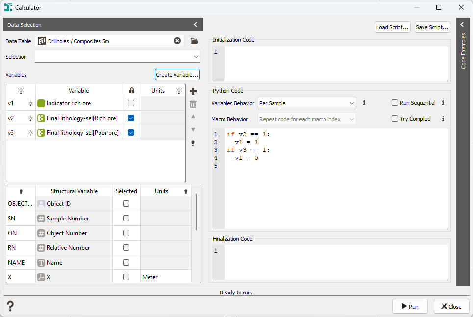
The Calculator enables you to create and set the value of variables in a given Data Table as being a transformation of other variables defined on the same table.

The user interface is split into three sections. The left section Data Selection gives access to the Input Data Table and Selection. The central part concerns the operations that would be run on the selected data. And the rightmost section presents Code Examples. Left and right sections can be shrunk/expanded.

Data Selection

• Data Table. Select here the data table you want to work with.
• Selection. You may apply a selection. The Python code will be used only inside this selection. Samples outside the selection will be left untouched.

• Variables. Two tables are shown. One for user-selected variables and another with the structural variables of the Data Table. The columns of the tables are the alias used during evaluation of the Python code, the real Variable name and the Unit used for variables that have a Unit Class. The aliases are used to make the syntax simpler and avoid problems with long names or with special characters. All aliases can be customized.

  • User-selected Variables. In the user-selected variables, you can add entries to select variables amongst non-structural variables. They can be of any type: Numerical, Categorical, Selection, Alphanumerical or Macro Variables. Aliases for user-selected variables are by default v[x] for variables and m[x] for Macro Variables (with x being the rank). A padlock column indicates wherever the variable will only be used for reading or for read/write.
  • Structural Variables. The list has a fixed size and depends on the selected Data Table. It contains all the available structural variables. The default alias for structural variables is all uppercase and corresponds to the role of the variable. An additional column indicates if the variable is to be used or not (say for memory reasons).

  • Create Variable. Click here to the create new variables in the Data Table to be used during the Python code evaluation.

    • Name. Specify here the name of the new variable.
    • Storage. Select one of the following type: Integer 32-bit, Integer 64-bit, Float 32-bit, Float 64-bit, Float 32-bit, Selection, Categorical, Text.
    • Unit Class. Define here the Unit Class for this variable (for Numerical Variables).

    See more in Create Variable.

Python Code Section

Three sections of code are available. The Initialization Code will be run only once. The main Python Code may be run several times depending on the type of calculation chosen. Finally, the Finalization Code is executed. All sections must be written in Python language.

• Initialization Code. The code will be executed once before the main code section. This code can be used to import some Python modules, define some functions, or initialize some global variables. Variables declared here will be made available to the main section code allowing these to be updated during each run of the main section. The code does not have access to variables defined in the Data Selection.

• Python Code. This code will be executed over portions of or over the entire data table contents. It gives access to the variables defined during Data Selection. Each selected variable of the selected Data Table will be available via its given alias. This means that if you assigned the alias v1 to the variable MyKrigingVariable, values from MyKrigingVariable will be set in Python variables named v1 and the code will be executed.

  • Variables Behavior: The number of samples assigned to the aliases variables will depend on the behavior chosen. All variables are read from the selected Data Table as the same time, stored in Python variables, code is executed, and values are written to the Data Table variables if they are selected for read/write.

    • Per Sample: The Python variables are assigned with the value of one sample at a time. v1 will sequentially take the value of the first sample and the code will be executed, then it takes the value of the second sample, etc... In fact, for performance reasons, the code will be vectorized in executed much less time than the number of samples in the table. This mode allows a simpler syntax than other modes because it considers only one sample and as such the value can be stored in a scalar variable.
    • Buffered Samples: The Python variables are assigned to a buffer / an array of input samples. You cannot control the number of samples available. In this mode, the variables are arrays (Numpy arrays) of the input samples. This mode allows more efficient computation but requires care: the variables are arrays and as such you will need to know more about Numpy.
    • Per Borehole: This mode is only available for Borehole Data Tables. It will process the sample of one borehole at a time. The code will receive the values of one borehole in the Numpy arrays corresponding to the selected variables. This mode allows the computation of some operation over all the samples of each borehole, like smoothing, completion,...
    • As Grid: This mode is only available for 2D or 3D Grid Files. The whole grid will be loaded at once and aliases will be populated with the values of the variables in 2- or 3-dimensional Numpy arrays. The indices of the dimensions of the Numpy arrays are the 0-based X, Y (and Z in 3D) indices. This mode requires the whole grid to be stored in memory, so it can consume a lot of memory. But it allows processing over the complete grid samples, like image filtering, having access to the neighboring samples,...
    • Whole File: All samples are available in one go (like in the Per Grid mode, but it also works for all other kind of Data Tables). A big Numpy array containing all the samples (ordered by Sample Number) for each selected variable. This mode can be memory-consuming but allows the computation of operations that require all the samples, for example to sort the data, compute quantiles,...
  • Run Sequential. When the reading/writing Mode only works on a subset of the data, the algorithm might run multithreaded and buffers of samples might come up in a different order from one run of the task to another. To ensure order of execution of buffer samples, check the Run Sequential mode. This disables multithreading and runs buffered operations on each block of data read from the file (sorted by Sample Numbers), waiting for the operation to complete to run the next block.

  • Macro Behavior. When macro variables are selected as input, you must define how realization looping will occur.

    • Repeat Code for each macro index. A list of indices common to all selected macro variables is established and the code is executed as many times as there are indices. Variables types remaining unchanged, meaning that for "Per Sample" mode, variable remains scalar variables; "Per Grid" mode will still use 2- or 3-dimensional arrays depending on the dimension of the file; and all other modes will receive one-dimensional Numpy arrays. Beware of modifications of standard (i.e. non-macro) variables in this mode: the commands are executed several times for the same set of samples.
    • Access macro indices in numpy array. Each Python variable will have an additional array dimension containing the indices of the macro variables. This means than for "Per Sample" mode, the variables will now be single dimension arrays, "Per grid" variables arrays will now have 3 or 4 dimensions (respectively for 2D and 3D grids, with the first dimension being the index); other modes will have 2-dimensional arrays, the first index being the macro index, the second being the sample rank.
  • Try Compiled. This option is only available in Per Sample mode. Native C++ code is automatically used behind the scene to gain computation time when simple transformations of numeric variables are applied on large datasets. This optimization is not activated when an Initialization or Finalization code is present, or when a non-numeric variable is used.
• Finalization Code. The code will be executed once after the different main code buffers have been treated. Variables created in the Initialization Code and updated during the main processing code will be available here for final treatment or printout. The code does not have access to variables defined in the Data Selection.
• Load Script. Use this button to load an existing python script.
• Save Script. Use this button to save the python script entered in the Text Editing Zone.

• Type Ctrl-F to bring up a Find-Replace widget across the bottom of the window:

  

  • Check the Match case option to do a case sensitive comparison (the string which you are comparing should exactly be the same as a string which is to be compared).
  • Check the In selection option to apply the search only to the highlighted lines.

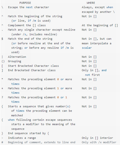
  • Check the Use regular expressions option to define a pattern you are searching rather than an exact string. You can search strings beginning with "selection", continuing with anything else and ending by "mesh", by using "selection.*mesh". The main expressions are:

    

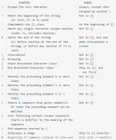
    For more details, you can also refer to this website.

  • Check the Search backwards option to search from back to top. The search always begins from the line where your cursor is.

  Click ESC to hide the Find-Replace widget and Ctrl-K to comment highlighted lines.

  This Find-Replace tool can be activated in the Python Code section or in the Finalization Code section of the Calculator.

Some useful keyboard shortcuts:

• Ctrl + K to comment the selected line(s).
• Ctrl + Shift + K to uncomment the selected line(s).
• Ctrl + F to find and replace.
• Ctrl + A to select all.
• Ctrl + C to copy.
• Ctrl + X to cut.
• Ctrl + V to paste.
• Ctrl + Z to undo.
• Ctrl + Y to redo.

Code Examples

This section, shrunk by default, can show you different examples using the different Variables Behavior mode to give you some real-life examples of operations.

Press Run to apply your script, or Close to cancel.