Compositing / Well discretization

Objectives

The Compositing / Well discretization or regularization is a well-known method for geostatisticians to get composites of the same size from an irregular boreholes / wells sampling.

Methodology

The algorithms involved in the compositing process are just a "weighted average" of the original property, the weights being the length of the analyzed samples that fall inside the new regular composites.

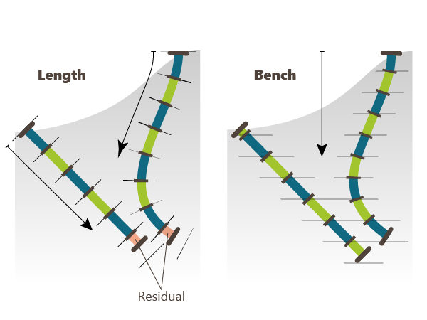
Compositing may be performed by Length or by Bench:

By length means that the composites have the same length along the boreholes
By bench means that the composites begin and end on the tops and bottoms of regular horizontal benches.

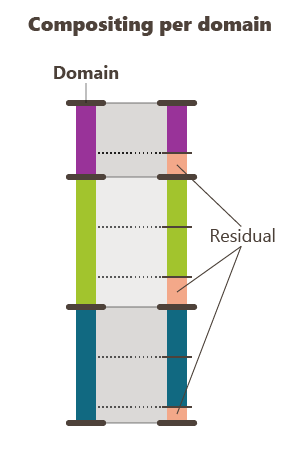
Note: When choosing to apply a compositing by length, a domain variable can be considered. It takes into account the boundaries between two domains (i.e. the limit between two samples for which the domain information is different) and keeps them unchanged after compositing. In other words, the compositing is made in a way that a composite always starts and ends on a boundary. The boundaries between domains are at the same coordinates before and after the compositing.

Input

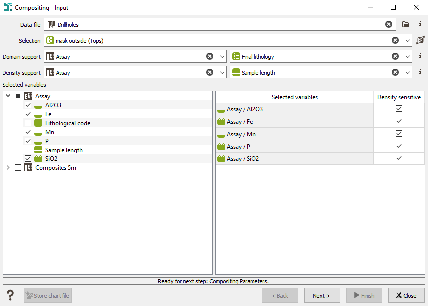
Select the boreholes Data file on which you want to apply the compositing.

Note: The boreholes file must at least have a table of Assays type. Markers and Logs tables or a Boreholes file are ignored because they are considered as points information and do not have a thickness.

A Selection on any data table from the boreholes file can be used as a filter.

All the data tables associated to the boreholes file, as well as their variables, are listed. Check here the ones you want to composite (you will find them in the composite output data table).

An optional Domain variable can be chosen. The domain variable may be located on any assays data table from the boreholes file. In this way the boundaries between two domains will be taken into account. The compositing will be made in a way that a composite will never cross a domain boundary.

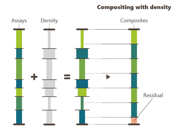
An optional Density variable can be applied. In this case, a Density sensitive column appears in the Selected Variables table. If the corresponding toggle is checked, the variable will be weighted by the density value during compositing (in addition to the weight by the length). The density variable must be defined for each input sample.

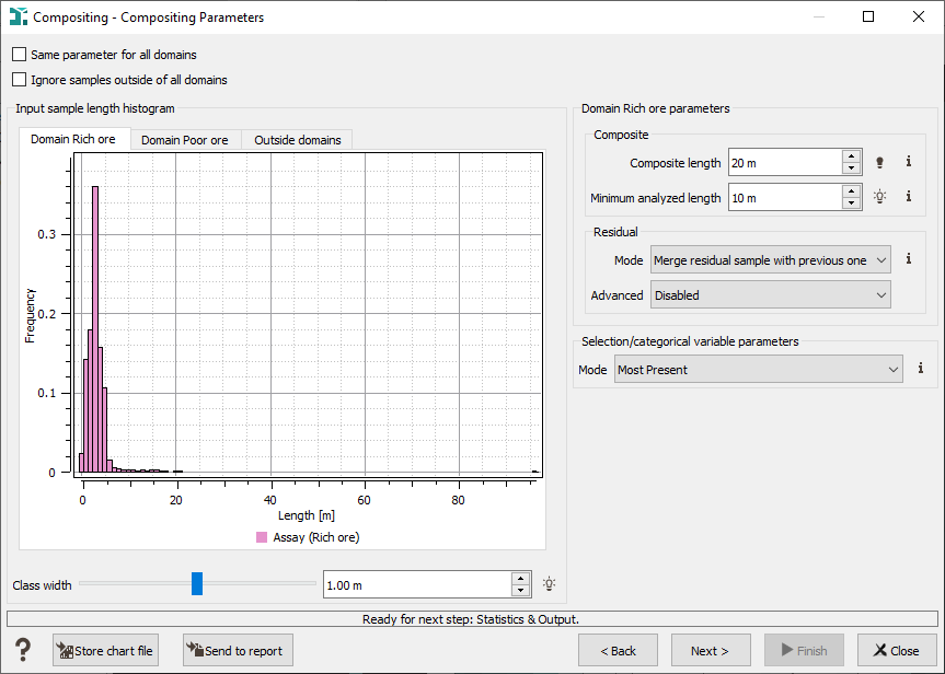
Compositing Parameters

The two following options are only available if a domain variable has been selected.

Same parameters for all domains: untick this option if you want to define different parameters for each domain. You will get a domain selector to customize compositing parameters in each domain.
Ignore samples outside of all domains.

Note: The method used when using domains is the compositing by length.

The histogram displays the frequency of the samples length corresponding to a Class width. This parameter can be customized using the slider or giving a specific length on the bottom of the interface.

The graphic can be saved in a Chart File clicking on the Store chart file button available in the bottom left of the interface. If several histograms are computed, in case of domains for example, all the histograms will be saved as charts at once.

If there is no domain variable selected, 2 different methods are available to compute the composites:

Compositing by length
Compositing by bench

Note: If your boreholes are mainly horizontal, the compositing by length will be preferred. Be careful about the choice you made.

Compositing by Length

Composite length: the composites will have the same length along the boreholes.
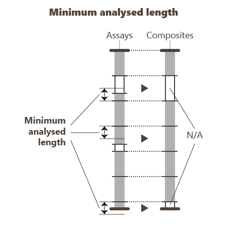
Minimum Analyzed Length: if the analyzed length of a composited sample is smaller than this value, the variable value will be set to undefined after the compositing.
Residual mode: if the last sample is smaller than the composited length, you can choose how to manage it for the final composited file.
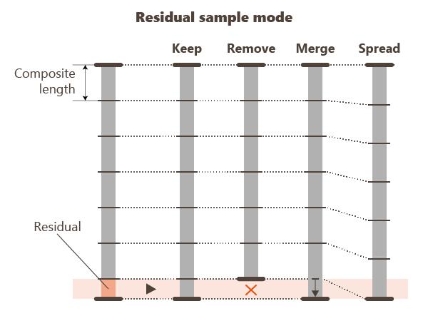
- Keep the sample as it is.
- Remove the sample.
- Merge the sample with the previous one. The residual sample is merged only if its length is inferior to Composite length / 2
- Spread the sample length on all the other samples of the boreholes.
Note: The merge and spread modes explain why the final compositing length visible in the statistics table can be different from the required composite length.
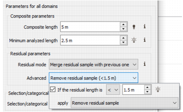
Advanced: this advanced parameter allows to manage the residuals regarding their length. You can apply one general mode for the residuals but another mode for particular residuals.

Example: The composite length is set to 1 m. The general residual mode is «Keep» and the advanced mode is «Remove if the residual is smaller than 0.25 m». In this case, a residual of 0.5 m at the end of a borehole will be kept whereas a sample of 0.1 m will be removed (because 0.1 < 0.25).

Compositing by Bench

Note: The Bench mode is not available in the case where a domain variable is set.

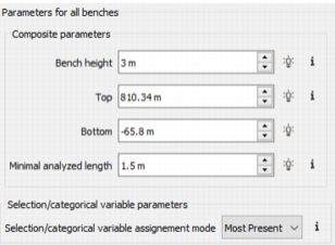
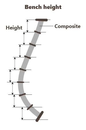
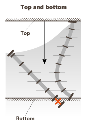
In this mode you have to specify the Bench Height, the Top and the Bottom of the compositing (the upper and lower levels between which the compositing will be performed).
Minimum Analyzed Length: if the analyzed length of a composited sample is smaller than this value, the variable value will be set to undefined after the compositing.

Selection/Categorical Variable parameters

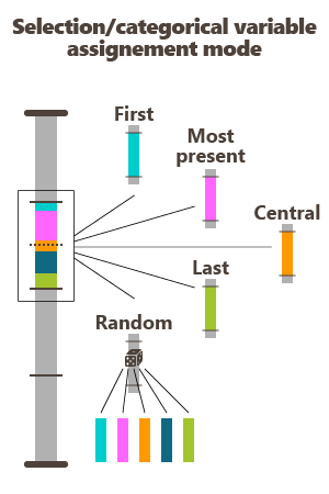
The chosen mode defines the category/selection to be assigned to the output composite samples. The different modes are as follows:

First: the category associated to the composited samples will be the one from the first sample of the composite.
Most Present: the category associated to the composited samples will be the most represented one.
Central: the category associated to the composited samples will be the one that is the closest to the sample gravity center.
Last: the category associated to the composited samples will be the one from the last sample of the composite.
Random: the category associated to the composited samples will be set randomly.

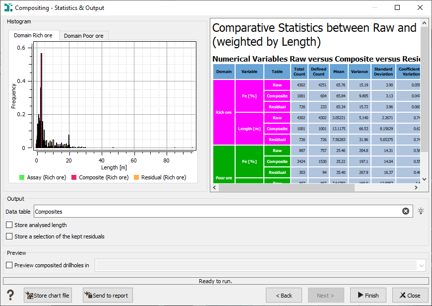
Statistics & Output

At this step, an histogram of the lengths (only with the Length mode) and a table comparing statistics on variables before and after compositing are displayed.

The histogram displays the lengths of the assays, the composites and the residuals (before any processing of them). If a domain variable was set, several histograms are displayed in different tabs.
Statistics on the assays, composites and residuals (before any processing) are computed on variables by category, if a domain variable has been applied. Variables are grouped in three tables for numerical, categorical and alphanumerical variables.

Note: The residuals statistics are only displayed when using the compositing by length. There are no Residuals with Bench mode.
The result of the compositing is saved under a new Data table, named «Composites Xm» by default, where «X» is the composite length. You can rename this new Data table as you want it.
The real Analyzed length of each composited sample (of each variable) can be saved in a dedicated variable. The program will create variables «Analyzed Length (var)».
A selection of the residuals can be saved in the output data table by ticking the Store a selection of the kept residuals if the Residual chosen mode was Keep. This option is allowed only in the case of the Length mode.
A Merged table can also be saved if several input Assay tables have been composited.
The composited samples can be visualized in a 3D scene before creating the new data table.

The histogram as well as the statistics table can be saved in a Chart File clicking on the Store chart file button available in the bottom left of the interface.