
Cross-Validation Options
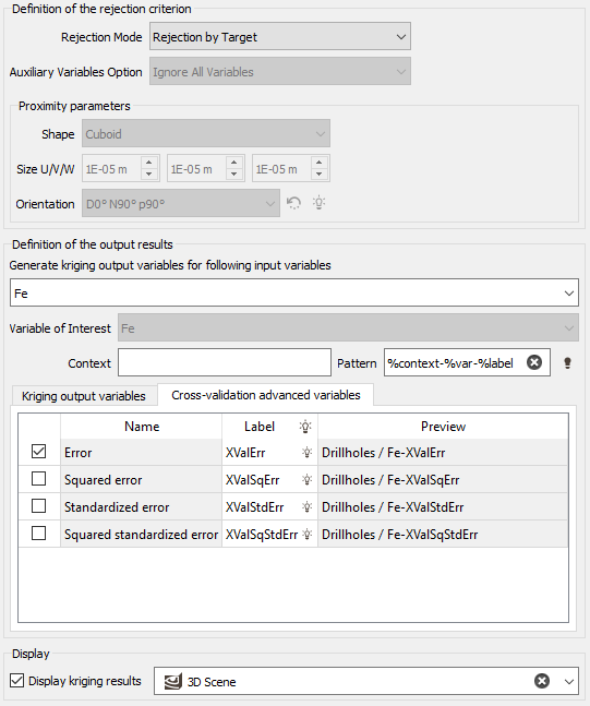
Definition of the Rejection Criterion
-
Rejection Mode: Different modes are available to reject one sample only or a more important part of the dataset.
- Rejection by Target: Use this mode to reject only one sample at a time.
- Rejection by Line: This mode is only available if the geostatistical set has been made from a borehole dataset. It will reject the sample we try to reestimate through the cross-validation as well as all the samples belonging to the same borehole.
- Rejection by Proximity: This mode will reject the sample we try to re-estimate through the cross-validation as well as all the samples located in a "neighborhood" around the target sample. The neighborhood is defined by a Shape (Cuboid, Ellipsoid, Elliptic Cylinder), a Size, i.e. a distance along U/V(/W) and an optional Rotation.
-
Auxiliary Variables Option: This option concerns the use of the information at the target point only in the multivariate case. The different possibilities are:
- Ignore All Variables: All variables are ignored. None of variables defined at the target point will be used in the cokriging process.
- Keep Auxiliary Variables: All defined variables are used except the Target Variable. All the variables defined at the target point will be used in the cokriging process, except, of course, the variable to be estimated.
- Keep Auxiliary Variables Only at Target Point: This option is available for collocated cokriging only. Only the collocated variable(s) defined at the target point will be used in the co-kriging process. Note that this variable has to belong to the data table and has to be defined beforehand in the Special Options page. It is obviously different from the Target Variable.
Definition of the Output Results
Generate kriging output variables for following input variables: By default, we will store the results associated to each data variable specified by the Input Geostatistical Set. Click on the Generate kriging output variables for following input variables selector to edit the variables list and deselect some variables you do not want to store their cross-validation results for.
The objective of the Pattern (and Context) parameter is to help the definition of output results names. You can edit this pattern to modify it and define the name of your choice. Click on ![]() to retrieve the default pattern: %context-%var-%label
to retrieve the default pattern: %context-%var-%label
The Label section is editable by a double-click for modification. The Preview enables you to see the final name associated to each output result.
You may then specify several output variables:
-
Kriging output variables:
- Kriging where the result of the estimation by cross-validation will be stored.
- Standard deviation / Variance: gives the associated kriging standard deviation / variance.
-
Cross-validation advanced variables: A list of additional variables corresponding to cross-validation statistics based on kriging results. These different types of errors are computed at the end of the run as the average quantities but also for each input point. They are useful to compare the experimental error (between the estimated and the true values) and the forecasted error within the model.
-
Error:

-
Squared error:

-
Standardized error:

-
Squared standardized error:

-
Where N designates the number of active points. In the previous formulae, the denominator involves the square root of the variance of the error which is usually equal to the kriging variance. However, when the target variable is characterized by a measurement error this term becomes:

The mean error and the mean standardized error measure the degree of unbiasedness. The most interesting quantity to analyze is the variance of standardized error which corresponds to the ratio between the experimental and theoretical variances.
What is remarkable about this quantity is that its numerator depends on all the parameters of the model except the sill, whereas the denominator is directly proportional to the sill. So, the model may be rescaled on the basis of the cross-validation results by multiplying the sill (or the coefficient of each basic model structure) by the variance of the cross-validation standardized error.
Another meaningful feature is to point out the data for which the cross-validation standardized error exceeds a certain threshold, that is, the outliers lying outside the corresponding confidence limit of a normal distribution. The points for which the cross-validation standardized error remains within this [-threshold ; +threshold] interval are usually called robust. By default, the confidence level is set to 99% which corresponds to a threshold of 2.5 (interval [-2.5 ; 2.5]). The confidence level may be modified according to the quantity and the quality of the information. For example, a confidence of 96% of the normal distribution will correspond to a threshold of 2.0, 68% to 1.0, etc.
Note: When the variogram model does not contain any nugget effect, a check is done before launching the calculations to automatically identify duplicate data points. The duplicate check is performed not only on the point coordinates but also on the values of the variables considered. A point is regarded as a duplicate if its coordinates are identical to another point and the variable values used for the kriging are defined.
This helps prevent matrix inversion instabilities that may lead to very bad results. In such cases, an error message will be displayed.
Graphical Results
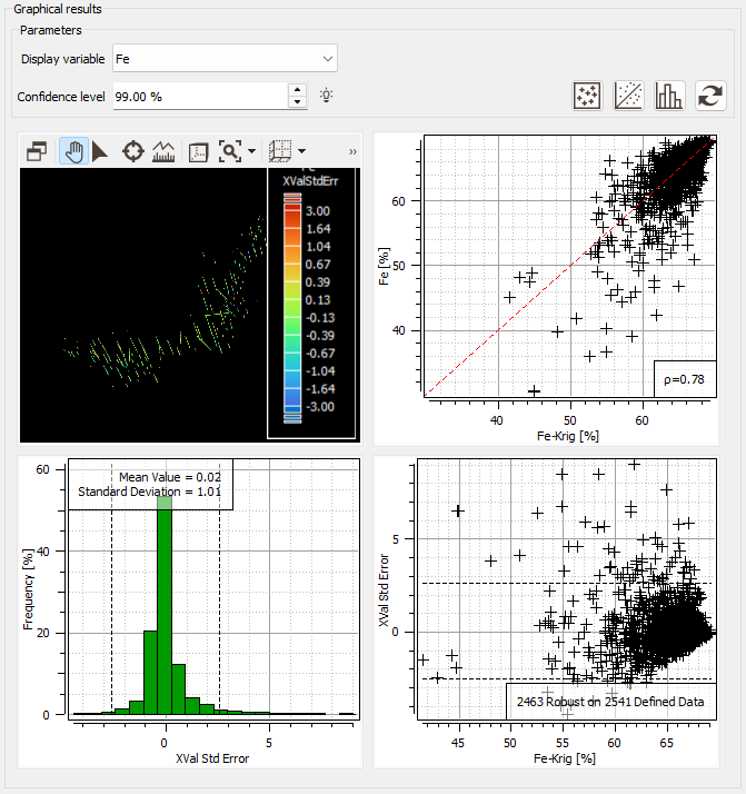
The different statistical results of the cross-validation are displayed in a graphic section in addition to the numerical results. It is composed of four views:
Enter the Confidence level which corresponds to the threshold value delineating the outliers from the valid points. The default 99% quantile of a normal distribution corresponds to a threshold of 2.5, that is, to the samples lying inside the 99% confidence limit of a normal distribution. This confidence interval will be plotted on the two bottom graphics (the histogram of the standardized estimation errors and the scatter plot of the standardized estimation errors versus the estimated values).
-
a Basemap (upper left corner) showing the location of the tested data points. The pattern dimension is proportional to the value of the true value Z and the color is linked to the error. Click
 to change the Color variable and the Size variable. These variables can be the Observed Value, the Estimated Value or the Error.
-
a Cross Plot (upper right corner) of the true values Z against the estimated values Z*. This cloud should be close to the first bisector. A point located far from the bisector corresponds to a value poorly re-estimated. However, it does not always correspond to an outlier. The variance of estimation may be large too and therefore, the standardized error still be close enough to 1. Click
 to:
to:- Swap Variables to interchange target and conditioning variables.
- Use Same Scale on Both Axis to have the same graduation following the X and Y axes. This option is useful when comparing two variables of the same nature.
- Draw Conditional Expectation Curve which plots the points representing the mean value of the target variable calculated for several ranges of the conditioning variable.
- Draw Standard Deviation around Expectation Curve which plots two additional curves which correspond to the expectation curve plus or minus the standard deviation calculated on the points of each class.
- Draw First Bisector Line
- Change the Number of Classes for the expectation curve
-
a Histogram (lower left corner) of the standardized estimation errors. It gives an idea of the unbiasedness (median of the histogram) and the quality of the estimate. It also helps locating the outliers which are outside the two vertical lines corresponding to the threshold value. Click
 to modify the Number of Classes.
The threshold value associated to the confidence level (applied on the standardized estimation error) is represented as two horizontal lines.
Remember that the variance of the standardized errors is a quantity whose numerator depends on all the parameters of the model except the sill whereas its denominator is directly proportional to this sill. The model will be rescaled on the basis of the cross-validation scores by multiplying the sill (or the coefficient of each basic model structure) by the variance of the cross-validation standardized error.
- a Scatter Plot (lower right corner) of the standardized estimation errors versus the estimated values Z*. Since the two variables are theoretically independent, this cloud should have no preferential shape. The threshold value associated to the confidence level (applied on the standardized estimation error) is represented as two horizontal lines.
-
If you change some parameters, graphics will not be consistent. In this case, they are greyed. Click
 to redraw the graphics.
- The four views contained in the Graphic results section are linked. All the objects react with the other ones. Highlight some samples in a graphic will highlight them in all the other graphics.
- When setting a multivariate Geostatistical Set, the Display variable list allows the selection of the variable that will be used for the graphics (by default the variable of interest). If you want to see the graphical results of another variable of your input geostatistical set, you should switch to this one in the selector and press the update button to redraw the graphics.
Display
Select the Display kriging results toggle to display the result of the Cross-Validation in a defined scene (2D or 3D) at the end of the run.
The generated graphics can be saved in a Chart File using this particular format (using the Store chart file button available in the task window).