Gaussian Variable
The ![]() Gaussian Variables item transforms a raw variable or residuals into a Gaussian variable. This transformation, also called anamorphosis function, is designed to:
Gaussian Variables item transforms a raw variable or residuals into a Gaussian variable. This transformation, also called anamorphosis function, is designed to:
- correct any strong asymmetry of the raw variable distribution and make the modeling of the spatial correlation easier;
- transform a Raw Variable into a Gaussian Variable (normal score transformation) that will be used in the simulation processes;
- calculate grade-tonnage curves.
Note: For detailed information about the methodology, please refer to the technical reference Gaussian Transformation: the Anamorphosis.
The anamorphosis will be saved in the Geostatistical Set and used for subsequent Kriging / Simulations process.
This item generates a tab to one side.
Many parameters can be customized. They are gathered in different sections according to their field of application.
-
Variable:
- With the selector, you can choose to work on the raw variable or on the residuals (if already computed).
-
A transformation can be applied: zero effect to activate it on the gaussian anamorphosis modeling if the variable contains a significant part of zero values (or lower than a very small value), standard else.
Note: The default value for the transformation is based on a comparison between the 10th quantile and the value 0.00001 (if the variable is positive). When the Q10 value is still below, the Zero effect is automatically activated.
-
Zero effect: In distributions with a large quantity of zero values for the experimental variable (or values at the detection limit of the measurement device for example), some problems could arise when dealing with its Gaussian transformation (relevant for, e.g., simulations and conditional expectations).
In the raw distribution, there are no issues with many zero values. They are considered as they are. When performing the anamorphosis step in order to convert the raw values to Gaussian ones, the same raw zero values are converted into different Gaussian values. The resulting variogram in Gaussian space therefore contains an undesired and artificial noise part.
Taking into account the zero effect appropriately processes the Gaussian values belonging to the lower tail of the distributions with a Zero Effect phenomenon. A truncated Gaussian variable is created and used in the variography step (when computing a Gaussian variogram). Thus, the Gaussian variogram model does not contain the artificial noise. When saving the Gaussian variable (through saving the geostatistical set), the lower tail is filled in with a Gibbs sampler.
For values less than or equal to: indicate a threshold for the values which should be considered as zero. The number of samples below or equal to the given value is printed, as well as the proportion.
Note: This section is only displayed if the Zero effect transformation is applied. This is not compatible with the Residuals.
Note: It is mandatory then to calculate a Gaussian variogram to take into account the zero effect in the anamorphosis.A special option in the Gaussian fitting window allows to display both the model on the experimental data, and the upscaled model.
-
-
Raw to gaussian transformation:
- Frequency: This is the simplest way to transform a raw variable: the variable values are sorted by increasing order and the Gaussian value corresponding to the same cumulative frequency is calculated. Two identical raw values get different Gaussian values. The Gaussian histogram is then perfect, when no weights are used. This is the recommended method, thus the default one.
- Interpolation: A linear interpolation of the anamorphosis model is used to inverse the function. Two identical raw values get the same Gaussian value.
-
Empirical: This is almost the same method as Frequency. The Gaussian values are calculated using the empirical cumulative distribution. However, with this method two identical raw value get the same Gaussian value. If the distribution of the raw values is not regular, with many zero for example, the distribution of the Gaussian variable can be different from a true Gaussian distribution.
Example: Raw values = 1, 1, 6, 8, 8, 8, 10, 12.
Gaussian values (Frequency) = -3, -2, -1, 0, 0.75, 1.5, 2, 3.
Gaussian values (Empirical) = -2, -2, -1, 1.5, 1.5, 1.5, 2, 3.
-
Anamorphosis:
-
Apply a Dispersion law (Normal, Lognormal, Beta) on the data in order to increase the variance of the output distribution.
Note: The Normal law is not compatible with the Zero effect activation.
-
Define the authorized interval with a Minimum raw value and a Maximum raw value. It will define the range of values the model can reach. Click on
 to set the bounds of this interval to the minimum and the maximum calculated on the variable.
You can also specify a minimum and a maximum value of your choice. The minimum you specify must be less than or equal to the variable’s minimum and the maximum you specify cannot be less than the variable’s maximum.
Note: The values of the Minimum raw value and a Maximum raw value also specify the values of the additional parameters (minimum and maximum) of the lognormal distribution and the beta distribution.
Note: Be aware that this is the interval on raw data that will be considered in the back transformation of the simulated variables into raw scale (it allows the minimum or maximum of the back transformed data to be different from those of the dataset).
- In the Variance increase box, enter the value for the global variance increase that will be obtained by distributing this increase over all the input samples. The default is set to the experimental (weighted) variance divided by the number of samples.
-
Note: The actual version of the Gaussian anamorphosis does not make use of the Hermite polynomials, they are only used for integration formula (in uniform conditioning for example). For this, the number of Hermite polynomials is fixed to 100, which corresponds to an expansion into polynomials of degree 99.
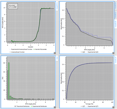
If you intend to use this anamorphosis function later for a back transformation after a simulation process, you should pay attention to the quality of the modeling and especially the intervals of definition. Moreover, six types of graphic representations are available. There are the anamorphosis transformation function, the experimental and modeled histograms and a set of four Grade-Tonnage curves (if the Display QTM Curves is activated on the top).
The two first curves (anamorphosis and histograms) are of general purpose:
-
Anamorphosis Function (Z/Y). This graphic view displays the anamorphosis function itself with the limits and the interpretation of the model. It is particularly useful for small datasets.
The anamorphosis model is represented with dot lines when outside the validity bounds called the practical interval of definition of the raw variable. These bounds are the points where the model is no longer smoothly increasing. The absolute interval of definition is represented as two horizontal lines. This is the Minimum Raw Value and a Maximum Raw Value defined by the user in the Parameters section.
- Histogram. The histogram of the data can be compared to the histogram derived from the anamorphosis.
-
The four other representations are related to grade variables and global reserve calculations:
- Mean Grade versus Cutoff (M/Z)
- Total Tonnage versus Cutoff (T/Z)
- Metal Quantity versus Cutoff (Q/Z)
- Metal Quantity versus Total Tonnage (Q/T)
These graphics refer to several quantities defined as below:
- Cutoff: successively equals the values of the variable (from the smallest one to the biggest one).
- Tonnage: this is the percentage of the samples for which the value taken by the variable is greater than the cutoff.
- Metal Quantity: this is the mean of the values taken by the variable which are greater than the cutoff. It is only defined for positive distributions.
- Mean Grade: this is the ratio of the Metal Quantity to the Tonnage.
Note: The two last icons Q/Z and Q/T are inactive when the dataset contains negative values.
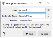
Click on the icon ![]() to save the calculated Gaussian variable. A window will pop up. To make easier the naming of the Gaussian, a pattern offers an automatic way to build the syntax of this name. This one is based on the variable name and on a defined label (Gaussian by default). We remind that Gaussian variables are also saved in the Geostatistical Set (which will be used as input of the Kriging / Simulation process). The action here allows the save of Gaussian variables without saving the geostatistical set.
to save the calculated Gaussian variable. A window will pop up. To make easier the naming of the Gaussian, a pattern offers an automatic way to build the syntax of this name. This one is based on the variable name and on a defined label (Gaussian by default). We remind that Gaussian variables are also saved in the Geostatistical Set (which will be used as input of the Kriging / Simulation process). The action here allows the save of Gaussian variables without saving the geostatistical set.
Note: It is not possible to only save a Gaussian variable using the Zero effect. The geostatistical set is mandatory.