
H-Scatter Plot
The ![]() H-Scatter Plot item is meant to analyze the spatial continuity of one or more variable(s).
H-Scatter Plot item is meant to analyze the spatial continuity of one or more variable(s).
In the univariate case, this functionality allows the plotting of a scatter plot between the selected variable and itself, that is the representation of all the pairs of samples whose locations are separated by a given vector. This vector is specified by its orientation and its elongation with a tolerance on both criteria. The coordinates along the X-axis and Y-axis are the two values of the variable at these two sample locations (see example below).
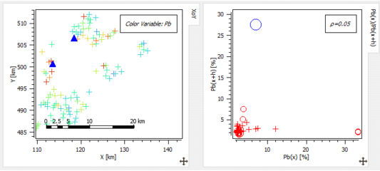
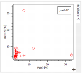
Note that this procedure is also valid for the multivariate case. In Isatis.neo, we are restricted to a bivariate case. For example, in the case of two variables entitled Pb and Zn, all the pairs {Pb(x);Zn(x+h)} will be represented where h fulfills the distance and orientation constraints (see example below).
- The Swap Variables option allows interchanging main and auxiliary variables.
-
Pair Selection: The H-Scatter Plot is a scatter diagram between the selected variable and itself. Each point on the graphic corresponds to a pair of samples such as their distance and orientation satisfy some constraints. These constraints are defined by:
-
the Calculation Mode: Two types of H-Scatter Plot can be calculated, omnidirectional or directional.
- Omnidirectional. No selection is performed on the pairs of samples according to any directional criterion. All the pairs are taken into account. The following parameters of Reference Direction, Tolerance on Direction and Radius will not be asked in this case.
- Directional. In this case, selection of samples is performed according to one defined direction. By default a Directional H-Scatter Plot is computed. If you have selected Directional, you have then to define a Reference Direction, a Tolerance on this direction and a Radius.
- the Reference Direction: Click Reference Direction to open the Define the Rotation dialog box and set the direction along which the pairs of points will be selected.
- the Tolerance on Direction: A pair of points will be taken into account in the calculations only if the angle between its orientation and the reference direction (on each side of the reference direction) is smaller than the Tolerance on Direction. Enter a value for the maximum angle between the reference direction and the orientation of the vector along the pair of points.
- Radius: It represents a cylinder lined up to the reference direction, out of which the pairs of points will be selected (as for the variogram). The value you will enter in the Radius box corresponds to the radius of the cylinder.
- Enter a Distanceh and an associated Tolerancet around this distance. Points of a pair separated by a distance whose value is included in this interval [h-t ; h+t] will be taken into account in the calculations. You can play with the
 /
/  buttons to add / to remove from the graphic a H-Scatter Plot associated to a different class of distances. Each cloud will be identified by a dedicated Color.
 - Variable Context: The H-Scatter Plot can be calculated in Univariate case (i.e. considering one variable), the default, or in Bivariate case (i.e. considering two variables). In the Bivariate case, the secondary variable can be defined from the same data table as the main variable (Bivariate in the Same Data Table option) or from a different one (Bivariate in other Data Table option).
- Define a Maximum Number of Outliers to display the n furthest points from the regression line as outliers.
-
-
Axes:
- Use log10 scale to apply a log10 transformation on the horizontal and/or vertical axes. Remember that the logarithmic scale can only display variable with positive values. When the option is activated, samples associated with negative values are discarded.
Note: When the option is activated, the correlation coefficient which is displayed is the one calculated thanks to the transformed variable.
- Use Same Bounds on Both Axes to have the same graduation following the X and Y axes. This option is useful when comparing two variables of the same nature.
- Use log10 scale to apply a log10 transformation on the horizontal and/or vertical axes. Remember that the logarithmic scale can only display variable with positive values. When the option is activated, samples associated with negative values are discarded.
-
Display:
- As you can display several H-Scatter plot associated to different distances and tolerances, you have to choose which one will be the Reference Distance for the following display options. The different lines (regression, mean lines, etc.) and display as image will be calculated for the selected Reference Distance.
- The program allows two different types of representation, the classical one (by default) draws a point each time the two variables are informed. The second one (Display as Image) uses a discretization of the graphic in cells, each cell being colored according to the number of pairs falling inside this cell. This representation is particularly meaningful when the number of samples is huge. The Image Resolution defines the number of pixels along each axis.
This item also calculates:
- the First Bisector Line. This option is useful when having two variables of the same nature if you want to analyze where they differ (for example, an estimated value versus the corresponding true value).
- the Linear Regression between the target variable and the conditioning variable (Y|X). The equation of the regression line is printed in the view label and in the description of the reported graphic.
- the Mean Lines which plot the mean on each axis and show the gravity center of the graphic. The mean values are printed in the view label and in the description of the reported graphic.
- the experimental Conditional Expectation Curve which plots the points representing the mean value of the target variable calculated for several ranges (defined regularly by the Number of Classes) of the conditioning variable.
- the Standard Deviation Around the Expectation Curve which plots two additional curves which correspond to the expectation curve plus or minus the standard deviation calculated on the points of each class.
- Symbols: In this section, you can easily change the symbol (form, size and color) of the different kinds of points displayed on the graphic (Normal, Outlier, Highlighted).