Estimation & Simulations

• Estimation & Simulations
  • Quick Interpolation
  • Kriging
  • Display
  • Uniform Conditioning
  • Simulations

In this last step of the Estimation per Domain application select the estimation methods to be performed: Inverse Distances, Nearest Neighbor, Ordinary or Simple Kriging, Uniform Conditioning, Localized Uniform Conditioning and/or Simulations and set the associated parameters.

Quick Interpolation

• Inverse Distances

  • Power: The inverse distances estimation is a linear combination of the neighboring information. The weight attached to each information is inverse proportional to the distance from the data to the target, at a given power.

    

    

• Nearest Neighbor: At each target point, the resulting value is equal to the value of the closest active data point contained in the neighborhood.

Kriging

Select the kriging method you wish to compute.

• Ordinary Kriging

• Simple Kriging

  • Global Means: In the current domain, the mean of each variable is considered as a constant value.

• Discretization parameters

  

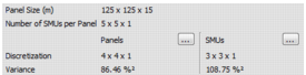
  • Panel Size (m): This parameter has been defined in the second step of the Estimation Preprocessing application during the Estimation Group Definition step.
  • Number of SMUs per Panel: This parameter has been defined in the second step of the Estimation Preprocessing application during the Estimation Group Definition step.

  • Discretization: It gives the discretization used for the panel or SMU kriging. Its values are optimized automatically.

    Click on ... to modify the discretization.

  • Variance: It is the Variance in between panels or SMUs. It is obtained by using the corresponding discretization and the Krige formula.

• Correction of Negative Estimates: This option replaces negative values in kriging results (Grade, Accumulation and Thickness variables) either by zero or an undefined value.

  Note: By default, negative density estimates are replaced by undefined values.

• Save Advanced Results for Classification: if this option is selected, the following Advanced Variables are stored in the panel sub-section of the results section:

  • Correlation Z/Z*: Stores for each panel of the grid the coefficient of correlation between actual value Z and estimated value Z* of the specified variable.

    

  • Covariance Z/Z*: Stores for each panel of the grid the covariance between actual value Z and estimate Z* of the specified variable.

    

  • Kriging Efficiency: Stores for each panel of the grid the kriging efficiency of the main variable. Where KE is the Kriging Efficiency, BV the theoretical variance of Panels within the domain (Panel Variance detailed above) and KV the Kriging Variance.

    

  • Slope of Regression Z/Z*: Stores for each panel of the grid the slope of the regression of the actual value Z knowing the estimated value Z* of the specified variable.

    

    Note: C00 means the covariance between the target point and itself. In the case of block kriging, Cvv (covariance between the target block and itself) is used instead.

  • Weight of the Mean: Stores for each panel of the grid the weight of the mean for the specified variable. Its value is derived from a Simple Kriging.
  • Number Neighborhood: Stores for each panel of the grid the number of samples used to krige each block.
  • Mean Distance to Neighbors: Stores for each panel of the grid the mean distance from block gravity center to samples used to krige each block.

Display

Tick the toggle to display kriging results in a scene.

Uniform Conditioning

Note: Uniform Conditioning is meant to calculate the recoverable resources in panels for a given SMU support. Localized Uniform Conditioning is a post-processing of Uniform Conditioning: the local grade metal tonnage calculated by Uniform Conditioning is preserved while the distribution of the grades for each SMU is guided by the rank of the SMU estimates.

• Cutoffs: Cutoff List defined in the first step of the Estimation Preprocessing application.

  The Cutoff List must be the same for all the estimated domains of a Partition for a given Estimation Group. If the user is working on the first domain of an Estimation Group the Cutoff List can be modified by clicking on . Otherwise, the Cutoff List is in read-only mode ....

• Localized Uniform Conditioning: This method is only available if the Uniform Conditioning is selected.

Simulations

The turning bands simulation technique is based on the simulation of a random function along 1D bands (with random orientation) which are then "combined" to produce the final simulation.

• SMU Discretization: It defines how many points are simulated per SMU, this number is calculated automatically. Increasing this number will increase the computing time.

  Click on ... to modify SMU Discretization Parameters.

• SMU Variance: It is SMU Variances in between SMUs. It is obtained by using the discretization and the Krige formula.
• Number of Simulations: Enter the number of simulations (of the same variable) to perform simultaneously. There is no theoretical limit on this parameter, except the performance of the working machine.
• Seed: Number used to initialize the Random Number Generator. Click on the dice to generate automatically random seed numbers.

• Number of Bands: Enter the number of turning bands to be generated by the simulations. The minimum and maximum authorized values are respectively 200 and 2000.

  Note that the quality of the simulation relies on that single parameter. Increasing this number will increase the computing time.

• Quantiles: This parameters is used to get a post-processing on the simulations. For each SMU, they are the quantiles of the N simulated values.

• Display Simulation Variograms: For validating the simulation process you can compare the input gaussian model to the output results. Click on this button to launch punctual conditional simulations of the gaussian variables and the computation of their experimental variograms. Experimental variograms are computed along the principal directions of the gaussian variogram model.

  The mean of simulation variograms and the variogram gaussian model are superimposed to the experimental variograms.

Press Finish to perform the computations.

All the results are stored in the Results section of the Resources Workflow Data tab.