
Variogram Parameters
This section groups the different parameters required for the variogram calculation: the experimental variogram and its associated model.
The variogram considers pairs of variables measured on two different samples. In the univariate case (i.e. if you select one variable), only one variable is considered in two different points. It enables experimental simple variograms (univariate case) or experimental cross-variograms (multivariate case, i.e. if you select several variables) to be plotted, that is to display the variability between the two variables versus the distance between the two samples. In addition, this procedure enables the set of pairs of variables being split into several families according to the direction in the space along which the pairs of points are aligned, and to calculate and display the variograms related to each family. These are the directional variograms. Here, in the particular case of a grid, the directional variograms along the main directions U, V and W will be displayed by default.
Variograms will be computed along two or three directions according to the dimension of the reference system 2D or 3D: U, V and W.
Note: U, V and W are the notations for the main directions of the rotated grid, i.e. the main directions X, Y and Z become U, V and W in the rotated grid.
The following parameters correspond to the calculation of the experimental variogram:
You can enter a Rotation to define a reference plane orientation for your input grid. By default the rotation is set to the grid rotation.
For each direction U, V and W:
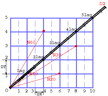
- Enter a value for the lag in the Lag Value box. The lag defines the variogram classes along the distance axis (horizontal). Each class is centered on a multiple of the lag. Only the pairs of points whose inter-distance equals a multiple of this lag (plus or minus the Tolerance on Distances) will be retained for the calculations.
- The size of the first lag, next to the origin of the variogram, equals lag-tolerance(lag) (half the lag value if tolerance is set to 50%).
- Define the Maximum Distance between two points beyond which no pair will be retained for calculations.
For each direction, the automatic values are initialized to have a maximum distance approximatively equal to the half of the grid size and a lag value in order to have 10 computed lags.
Note: In calculating the variogram for the first lag, a pair of points will contribute if their distance in the calculating plane is included between the values lag-tolerance(lag) and lag+tolerance(lag), where lag denotes the value of the lag and tolerance(lag) is the tolerance on the lag.
The procedure allows you to fit a model on the experimental variogram(s). This procedure offers some automation to help you performing the fit. Nevertheless, it is strongly recommended to check the fit quality using the different graphical possibilities.
Click the Automatic Fitting Parameters to access the automatic parameters of the variogram model (including the Nugget Effect value, the normalization and the set of structure(s)).
-
The Normalization option enables you to normalize the sill of the simple variograms to the experimental variances or to the correlations for the cross-variograms. Two modes are available:
- During Automatic Fitting: this mode automatically adjust the experimental curve by honoring the experimental variance (the sum of the sills will be equal to the variance).
- Post Automatic Fitting: this mode automatically adjust the experimental curve and rescale after the sills to the experimental variance.
- Click the Advanced button to access the automatic fitting advanced parameters. The automatic fitting algorithm is made to minimize the distance between the model and all the different experimental variograms for any calculation distance. The automatic fitting procedure helps you adjust the model by calculating optimal sills, ranges and anisotropies from any set of basic structures. We define a Maximum Number of Iterations to test to meet the minimization criterion. If the criterion is not attended, an error message to say that the algorithm failed the fitting will be printed. The Reject Criterion represents the percentage of variance below which a structure will be discarded.
-
Select the Structures on which you want to base your automatic fitting. Click
 to initialize the structures with the ones defined by the Setting up Preferences. By default in Isatis.neo, a cubic, a spherical, an exponential and a linear, plus a nugget effect are defined (the default structures are different in the Mining edition with two spherical structures). The SPDE button allows the use of structures compatible with the SPDE methodology (i.e. Mattern structures).
These are the most common sets of structures. If you want to use other structures, play with the
 and
and  to add / remove structures. The order of the defined structures also influences the result of the fitting. Use the arrows to modify the order of the selected structures. The Automatic Fitting procedure can discard a given structure, if this given structure does not improve the fitting. The Maximum Number of Structures can be used to enter a bigger number of structures but keeping only a reasonable number of these ones.
An echo of the structure type (as well as the nugget effect) and the maximum number of structures is printed in the main interface.