
Sensitivity Analysis
It is useful to understand how changes to schedule inputs affect the optimization workflow.
Understanding the risks and opportunities of your project is key, and by analysing your strategic plan's sensitivity to optimization parameters you can make more informed decisions about how your schedule and the intermediate data stages should be calculated.
Studio NPVS lets you set up a batch run of scenarios to compare outcomes where changes are made to key scheduling parameters including financial influences such as commodity price, mining cost, processing cost and recovery cost. Your optimization results will also be sensitive, potentially, to geophysical constraints such as slope angles and changes in stockpiled materials, for example.
Setting up a batch run is straightforward; first, define a base case with all parameter settings. Then, for each sensitivity analysis, define alternative values for one or more parameters.
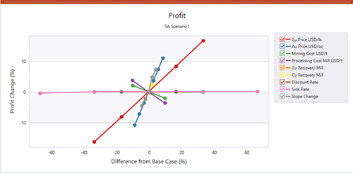
An example of a Sensitivity Analysis chart showing results for profit
For example, a base case is defined that describes the initial run's default parameters, such as product price, mining cost, sink rate, slope range and so on. In the base case, the copper price ($/lb) is 4.0. The schedule is then solved to provide the optimal extraction sequence based on this commodity price in conjunction with the other scheduling parameters (financial, physical, operational etc.). You want to see the impact on the schedule should copper fall to 3.0, so a sensitivity run is defined with only the commodity price altered.
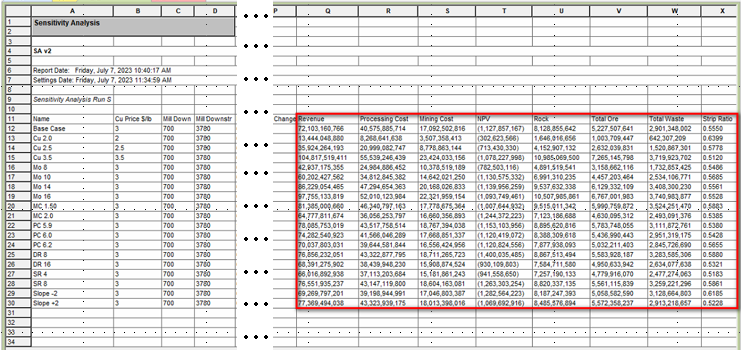
You can then compare the tabular results via a summary report indicating comparative revenues, cost, NPV, ore and waste fractions and strip ratio for each sensitivity scenario. Results can be viewed graphically too, using the Group Chart function that presents useful spider charts highlighting the impact of setting changes on other elements of the schedule.
One a sensitivity batch run has been prepared (see below) and executed, results are displayed as a summary report showing the inputs per scenario and their corresponding results. In the example below, the run results are highlighted and not all parameters are shown:
A dedicated Sensitivity Analysis summary control bar hosts this summary information.
Prepare a Sensitivity Batch Run
To prepare and execute a batch run to analyse scenario parameter sensitivity:
-
Use the Project Map control bar to choose a base case (right-click >> Sensitivity Analysis), from which other parameter values will be applied, to test the schedule's sensitivity to changes.
-
A copy of the scenario appears. Activate it (right-click >> Case Study >> Select).
-
In the Tasks Pane, expand the Sensitivity Analysis section.
-
Define the base Economic Settings for the sensitivity analysis batch run. These settings determine how the economic model is calculated and includes general Options, Prices, Mining costs, Processing costs and per-bench Adjustments.
-
Define the base Ultimate Pit Settings for the batch run, including options for Time, Ultimate Pit, Sequencing, Slopes and general ultimate pit Options.
-
Define the batch run configuration Settings; the number of runs to complete and, for each run, which parameter value(s) will overwrite the base case to see the impact of those changes on optimization results. See Create a Sensitivity Analysis Run.
-
Click Run.
Batch processing begins. Economic Model and Ultimate Pit calculations are performed for all scenarios. You can see how processing is progressing by displaying the Batch Run Log window, for example:
-
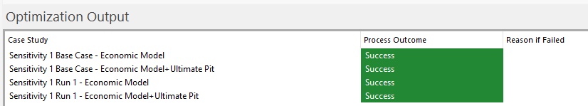
Once processing completes, messages may appear if particular scenarios could not be completed (say, the KPI for their base case was zero).
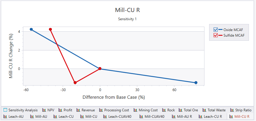
The Sensitivity Analysis chart results are also displayed in the Reports window, with each analysed parameter displayed as a different data series. For example, in the image below, the Processing Cost percentage change is shown for each parameter value (in this case, oxide and sulphide mining cost adjustment factors were analysed for values above the base value (oxide) and above and below the base case (sulfide):
-
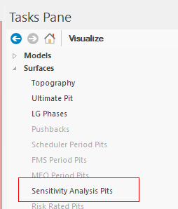
You can visualize the surfaces generated by a sensitivity analysis run using the Visualize section of the Tasks Pane:
-
The Choose Surfaces popup displays. This lets you pick the surface wireframes to generate to visually compare the outcomes of parameter changes in the 3D window. Pick the surface(s) you want to view and click OK.
Surface generation occurs. This can take a few minutes to complete, depending on the number and amount of data to be rendered.
-
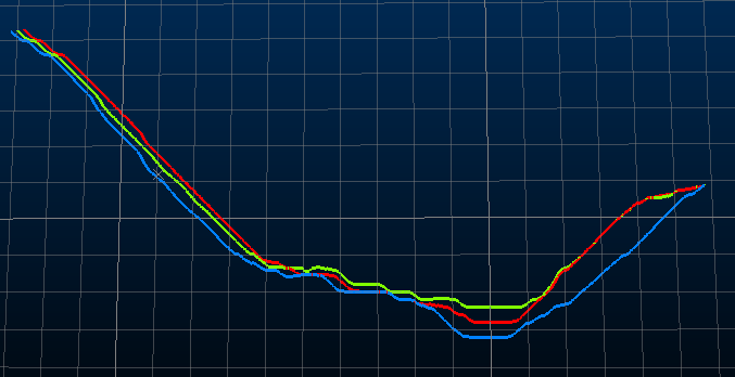
Once generated, surfaces appear in the 3D window and can be rendered as any other 3D optimization result. For example, the image below shows the 3 results for varying cost adjustment factors for sulfide (in the case below, the red line is the ultimate pit generate where MCAF is 1, green = 1.125 and blue = 0.75. The wireframe is rendered as an intersection with a N-S section:
Parallel Processing
Computing the optimal extraction sequence is a processor-intensive activity, so your application will make use of multiple cores if they exist, and you choose to use them. You set the number of maximum cores to utilize (if available) in Default Project Settings before you embark on a batch run. This allows multiple calculations to be performed simultaneously if system resources are available, reducing the time take to produce comparative scenario results.