Create Grade Shells

Activity steps:

A typical approach for using this command is:

1. Load a desurveyed drillholes file.
2. Launch the command.
3. Define the scope of your modelling; select the loaded Drillholes object and the Column containing grade values to be modelled.
4. Define the cut-off gradeValue to be modelled.
5. Choose how absent data values affect the generated grade shell, using Ignore absents:
   • If checked, absent grade values are treated as if they aren't there, so won't affect the generation of grade shells representing a cutoff.

   • If unchecked, absent grade values are considered to be zero grade, influencing the shape of the grade shell.

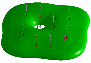
     For example, in the following image, Ignore absents is unchecked, and one of the holes contains only absent data as a result of a sample desurveying error:

     

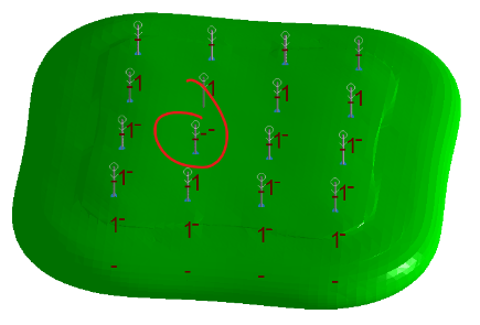
     For the same scenario, if Ignore absents is checked, the drillhole is ignored entirely, and the surface is interpolated throughout the absent data:

     

6. Specify your confidence in the accuracy of input sample data and associated contact points using Uncertainty. This can be set at a Default (meaning global) level, or read from a data attribute in the loaded Drillholes object. See Data Uncertainty.

7. A flat plane is required to calculate the resulting categorical volume(s), although it can be at any orientation. This is the mean plane of positive samples in the input set and is calculated automatically by default, but you can override this default using the Section Controls provided.
   • Interactively position the plane used to generate surface data by enabling the Section Editor control. See 3D Section Widgets.
   • Alternatively, modify the section using one of the controls in this section. These are replicated on the 3D View ribbon and Navigation toolbar.
   • Automatically align the view to be directly at the 'best-fit' plane through the data by enabling Auto look. This doesn't affect the definition of a modelling section - only the view is adjusted.
   • Align the view with a custom section.
   • Reset the modelling section to the automatically-calculated best-fit plane.

8. To define a trend to impart a guiding direction or directions throughout your structure:

   • Choose Default from holes to let Studio calculate the most appropriate trend for your data, using a consistent directional trend throughout your data. In effect, this makes use of a single, global search ellipsoid to interpolate a surface between contact points.
   • Choose Custom to define one or more ellipsoids that will be used to govern uni- or multi-directional trends throughout your data.
     1. Choose an existing ellipsoids data object, if one exists (if not, one will be created shortly).

     2. If appropriate, select Pick Drillhole Samples and select one or more drillholes that will be used to automatically create an ellipsoid. This is usually a set of holes within which a single trend is obvious. Once selected, choose Create Ellipsoid from Selected Data.

        The generated ellipsoid displays at the centre of the selected drillhole set.

     3. To manually position and define the axis dimensions of an ellipsoid, choose Create Ellipsoid. See New Ellipsoid.
     4. Edit any previously-created ellipsoid by clicking Edit Ellipsoid. See Edit Ellipsoid.

   • Ellipsoids are interpolated throughout the sample data in a uniform 3D grid, gradually morphing between defined ellipsoid shapes.

     Preview this grid by first selecting how detailed your preview will be (for example, 3 x 3 x 3 shows a grid of 27 ellipsoids, each in their interpolated shapes and orientations). Then, click View to render a temporary preview of ellipsoids on the screen, for example:

     

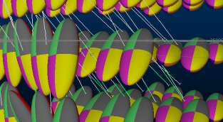
     From here, you can see how each part of the data is likely to connect to neighbouring parts.

9. Implicit surface modelling is an interpolative process where surface data is fitted (as closely as trends and other modelling parameters permit) to contact points. Enabled by default, the Snap to contacts section can enforce a secondary deformation of the generated surface to enforce a closer relationship between the output surface and its contact points.

   For more information, see Snapping to Contacts.

10. Define Surface Generation Controls:
    • The categorical modelling command needs to subdivide positive samples into smaller units to ensure ellipsoid centroids are positioned at suitable positions within the data set. You can choose to Subdivide automatically (Auto) or by choosing your own Fixed subdivision distance, where smaller values tend towards increased processing, but potentially a more representative result.
11. Define the Resolution of your output wireframe using the drop-down list (high values = small triangles = longer processing). For more precise control, select <custom> and enter your own value.
12. Choose how far beyond the hull of sample data categorical models can extend. You do this by entering a Percentage extra value, where 50% will allow models to extend beyond the cuboid hull of loaded sample data by up to 50% more, for example. As a worked example, if the bounding cuboid of data is 10 x 20 x 30 meters, the permissible 'space' for categorical modelling is within a cuboid 15 x 30 x 45 meters.
13. Decide if you want to constrain values that terminate at the collar (First), end-of-hole (Last), Both ends or Neither, using the Constrain ends drop-down list.
14. Define an Output Surface name. This is the name of the object to be created. If an object of the same name exists, a unique numeric suffix is applied.
15. Choose to either generate a new data object, or update an existing one:
• Click New Surface to create a new output wireframe object with default formatting.
• Click Update surface to replace a target object (of the same Surface name) with new data.
  • If Retain output formatting is checked, any previous overlay customizations to the existing model will be retained. That is, only the shape of the target object can change, not its visual formatting.
  • If Retain output formatting is unchecked, default wireframe model formatting is reapplied to the target object and any prior overlay customizations are lost. This cannot be undone.
16. Review your output volume.

Tip: Restore the settings from the last modelling run using Reset.