
Optimise Cell Size and Decluster Data
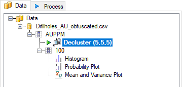
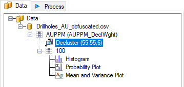
- Insert the Decluster component by right-clicking the AUPPM component in the Project Tree and selecting Add » Decluster from the menu. Your Project Tree should now look like the image below.
Note: The Decluster component will always be blank and require updating when it is first inserted. However, the cell sizes need to be optimised before this is done.
- To determine the optimal cell size for your data, you will first need to enter a minimum and maximum cell size value, as well as the step size that Supervisor will use to calculate points between them. This needs to be done for the X, Y and Z axes.
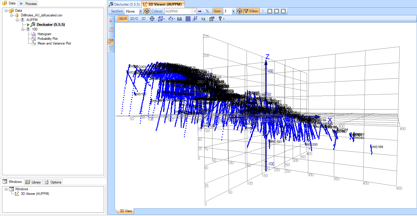
To get a starting point for these values, assess the data in the 3D Viewer to see how much it varies in each direction. In this dataset, the data on both the X-and Y-axes varies from approximately 0-400, and the Z-axis varies from approximately 0-225.
Using this information, we know that if we were to set the decluster cell size to X=400, Y=400 and Z=225, all of the data would fit in a single cell, which would be the equivalent of not being declustered at all. So, we need to find a cell size that fits within this grid and gives us the most equal weighting of points across the entire grid.
- Return to the decluster component in the Main Canvas and enter the following data into the Cell Sizes fields in the Optimise section of the Decluster tab in the Property Panel.
Axis Min Max Step X
5 80 5 Y 5 80 5 Z 2 10 2 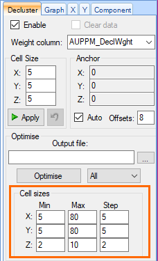
- Click the Optimise button above the cell sizes on the Decluster tab.
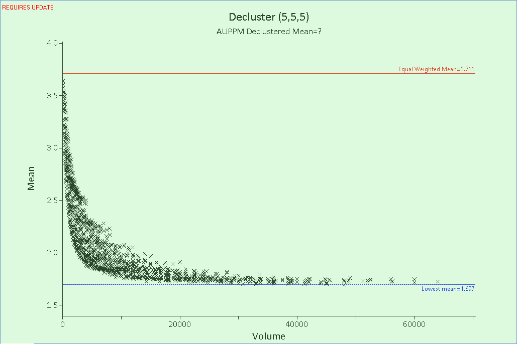
Supervisor will process all of the possible cell sizes and plot the data in the Main Canvas. The Decluster component still remains green and requires updating at this point, since the declustering process is not yet complete.
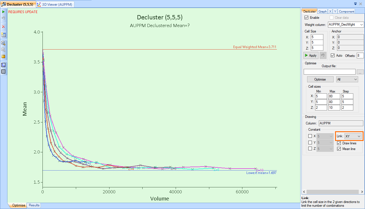
- In its raw form, the cell size data can be overwhelming, so we recommend linking two of the axes to make interpretation easier. Link the X- and Y-axes by opening the Link menu the Decluster tab and selecting XY.
The plot in the Main Canvas now only displays a single line for each potential Z-axis size, as shown in the image below.
The effect of declustering (in this example) shows a decrease in the mean as the higher grade samples are given less weight relative to the lower grade, sparsely distributed samples, until a point at which the cell size is big enough that the weighting returns to equality. This is logical, as a minimum cell size in which each sample is within it’s own cell, gives each sample an equal weighting, while at the maximum cell size, where one cell encompasses the entire region, each sample is also given an equal weighting. Since we are generally looking for a point just beyond the ‘elbow’ of this chart, if the data were all to trend downwards without inflecting upwards or levelling out, then the X and Y Max values would need to be increased.
Notes:
This data is from a deposit in which the high-grade samples are clustered. For deposits which have highly clustered low-grade samples, you would expect to see the data trend upwards and then back down.
See our article on Cell Size Optimisation for more background information on this process.
- Expand the plot axes by clicking and dragging them, to make it easier to see the points around the elbow in the data. The point that represents the most appropriate cell size is generally the point closest to the lowest mean (blue dashed line), close to the elbow. For this plot, select the point on the purple (Z=6) line, as shown in the image below.
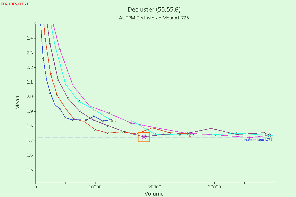
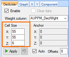
- Clicking a point automatically adds the cell dimensions to the Cell Size fields at the top of the Decluster tab. These fields should now read X: 55, Y: 55 and Z: 6.
-
Click the Apply button, beneath the Cell Size fields, to apply the newly weighted cell sizes to the data.
The optimised cell size values display next to the Decluster component in the Project Tree.
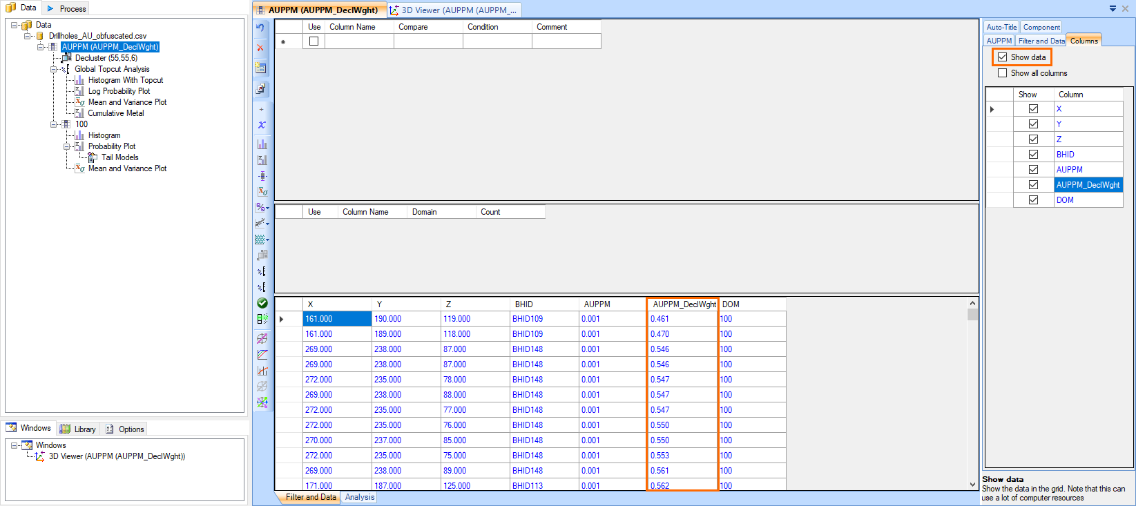
- The declustered values are applied as a weighting to the original data. The declustered weight column (AUPPM_DeclWght) can be viewed by selecting the parent component, which is the AUPPM assay in this case, and selecting the Columns tab in the Property Panel.Check the Show data setting at the top of the Columns tab in the Property Panel to view the individual points in the table.
The declustered weight field is automatically applied to all child components of the declustered component.
| «Previous |