Charts

• Charts
  • Contact analysis
    • General definitions
    • Algorithm
    • Parameters
  • Transition probabilities
  • Border effect
  • H-Scatter

All the views of all the graphic pages are displayed in this section, organized in several tabs corresponding to a dedicated perspective:

• Contact analysis,
• Transition probabilities,
• Border effect,
• H-Scatter.

Contact analysis

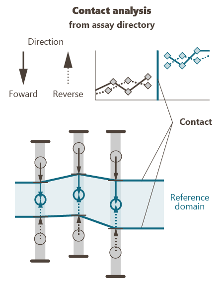
The Contact analysis section is designed to help you defining the type of contact between one domain and the others.

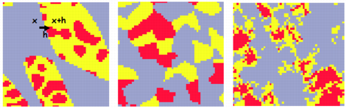
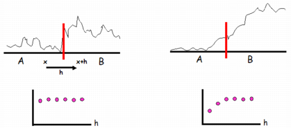
To do that, it calculates the mean value of a selected variable as a function of the distance of the samples in a domain to the contact with another domain. This calculation can be done considering all directions (omnidirectional) or choosing a reference direction. The mean value is calculated on samples, classically along drillholes, by distance classes. The display corresponds to the variation of the variable when crossing the domain borders from a targeted domain to the other ones.

The results will inform you about the variation of the variable of interest. Then, you will be able to determine if it is a sharp contact (brutal change of the variable values) or a progressive one (gradual variation of the variable values). In the case of a very progressive contact, you may create a “transitional domain” between the two studied domains.

General definitions

• Reference direction and distances

  The algorithm calculates the distance considering a reference direction between the core gravity center of a sample in a domain and the contact with a second domain. This distance is:

  • positive if the sample lies before the contact in the reference direction,
  • negative if the sample lies after the contact in the reference direction.

  

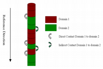
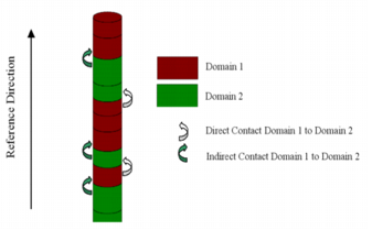
• Oriented contact

  Statistics are calculated in the chosen reference direction and in the opposite direction. The way of scanning the drillholes is important. The following figures show two configurations with different deference directions.

  Considering the contact from Domain 1 to Domain 2:

  • a direct contact is a transition from Domain 1 to Domain 2
  • an indirect contact is an inverse transition (i.e. from Domain 2 to Domain 1)

  

Algorithm

A given sample (located in the Reference or Target domain) will be taken into account in the calculations if:

• All the samples (along the reference direction if directional) between itself and the contact are within the same domain (Target or reference domain),
• The distance (in the reference direction if directional) between the sample gravity center and the contact is smaller than the distance between the sample gravity center and the closest sample in another domain.

Note: A sample located between two contacts will be taken into account only with the closest contact.

Parameters

• Domains: This section is common and shared by all the perspectives. It lists all the domains defined by the Domains definition variable in input. Select the different domains you want to take into account and define which one will be considered as the Reference domain. Samples belonging to not-selected domains will not be taken into account for the calculations.

• Distance:

  • from assay trajectory: This mode is only available when the input data table is an assays data table (on a drillhole file). Using this mode, the distances to the domains are computed along the drillhole trajectories.
  • from envelope of: This mode is the only one available if you select any input data file which is not an assays data table. In this case, the distances are computed regarding the envelope of a wireframe file (considered as a domain). The distance is calculated considering the shortest distance between the selected point and the intersection point with the mesh along an oriented line (following the reference direction). Select the wireframe file and the different objects, if several, you want to consider. By checking the Filter outside domains option, activated by default, the samples outside the selected domains are not taken into account.

  

• Display options: Optional displayed statistics.

  • Non-oriented curve: This option is only available when defining a reference direction (directional orientation). Check this option to consider samples regardless of the direction path (i.e. merging samples of the forward and reverse curves).
  • Global mean: display the statistical mean of the grade variable of interest in each domain, represented as a dashed horizontal line.
  • Number of samples: display on the graphics the number of points belonging to each class as text.

• Print:

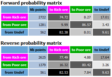
  • Print probabilities matrix: Activate this option to send probability matrix in the Messages window. This result allows you to easily interpret contacts between domains to define the lithotype rules in the Pluri-Gaussian Simulations for example.

  

• Output domain selection: Creation of an output selection. The selection is made using the distance between the target domain and the samples location. Three definition modes are proposed:

  • Hard boundary: selection of all the samples whose category corresponds to the target domain.

  • Oriented soft boundary: selection of samples according to the distance between the samples and the target domain. The distance can be defined interactively by moving the big red square from left to right on the graphs.

    • Forward distance: distance at the domain contact along the drillhole in the forward direction (from top to bottom).
    • Reverse distance: distance at the domain contact along the drillhole in the reverse direction (from bottom to top).

  • Non-oriented soft boundary: distance definition regardless of the direction path.

    • Distance to contact: selection of the samples which are closer to the contact than the chosen distance.
• Output selection pattern: name of the new selection that will be created in the input data table. A default pattern Boundary_%domain helps you defining the output name.

Click on Save to create the output domain selection.

Transition probabilities

The probability to enter a domain B when leaving a domain A depends on their connectivity:

• The “non-oriented” transition probability from a domain A to another domain - samples at x+h being inside A and samples at x being outside A - is represented by the variogram of the indicator of the domain A. The “non-oriented” transition probability to enter in B when leaving A as a function of distance h is:

  

  

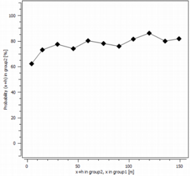
  This probability can also be normalized (by checking the Normalize curves option - ON by default) by the following value:

  

  When the normalize option is on, the graphic do not display anymore a probability but a ratio of probabilities. In some case when the probability to be in A or B is very low, the curves are very flat. When the normalization is on, it is easier to interpret the shape of the curves.

• We can also calculate the “oriented” transition probability. We obtain a non-symmetrical curve and the probability for negative distances. Instead of using the variogram of the domain, we calculate the non-centered covariance to enter from a domain A to another domain - samples at x+h being in A and samples at x being outside A:

  

  The transition probability from a domain B to a domain A is:

  

  

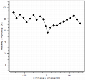
  Note this probability can be normalized (by checking the Normalize curves option - ON by default) by the value:

  

  When the normalize option is on, the graphic do not display anymore a probability but a ratio of probabilities. In some case when the probability to be in A is very low, the curves are very flat. When the normalization is on, it is easier to interpret the shape of the curves.

• Check Along assay trajectory to restrict the variogram/covariance calculations to samples belonging to the same drillhole only. This option is only available if the input data table is a drillhole file and is OFF by default.
• Use the option Oriented to compute the Transition probabilities using h or -h according to the orientation of the direction. In this case, calculations are made using the covariance function (not the variogram). If Oriented is switched off the orientation of the direction is not taken into account which means that only positive h are displayed (there is no distinction between h and -h). This option is not available if the input data table is a grid file.
• Tick Number of pairs to display the number of pairs involved in the determination of each point of the variogram/covariance curves (for each lag). The display is possible as text or as histogram using the selector.

Note: Samples that are not part of any domain are ignored.

Border effect

The Border effect section is meant to evaluate the impact of the domaining on the spatial variability of the input grade variable Z.

We consider that a deposit is divided into several domains D1, D2, etc., each domain being considered as homogeneous (stationary), except perhaps at borders, and is characterized by its geology, mineralogy, etc. and from a geostatistics point of view, by:

• its mean grade(s) Z(x),
• its structure: variogram,
• and the relations to its frontiers and to the outside (behavior at borders).

The application calculates spatial statistics based on variograms for each domain or pairs of domains:

• Mean [Z(x+h) |Z(x)],
• Mean difference [Z(x+h)-Z(x)].

All these statistics are derived from experimental variograms or ratio of variograms calculated from pairs of samples that are separated by a given distance h.

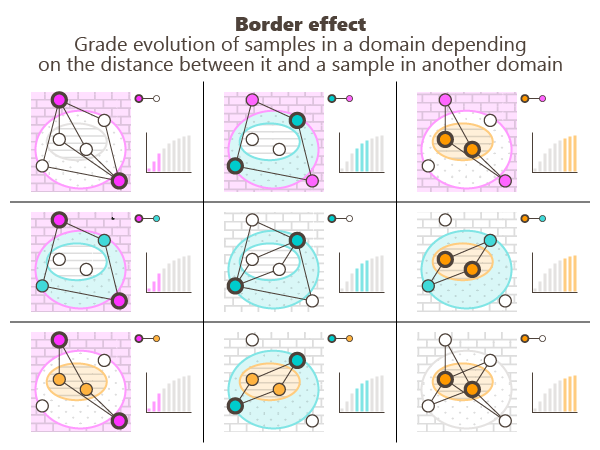
The results are displayed in a matrix, the rows being related to samples at locations x while the columns are related to samples at locations x+h:

• On the diagonal we have the probability of x+h in a domain D and x is in another domain,
• Out of the diagonal the probability of x+h in a domain e.g. D2 when x is in another domain e.g. D1 (probability of entering D2 (column) when leaving D1 (row)).

• Mean [Z(x+h) |Z(x)]

  • Border effects in a domain A can be depicted by the mean of Z(x+h) at x+h - when x+h is inside domain A while x is outside domain A - as a function of distance h as (graphics displayed on the upper-left/lower-right diagonal):

    

  • Border effects in a domain A close to a domain B can be depicted by the mean of Z(x+h) at x+h - when x+h is inside domain A while x is inside domain B - as a function of distance h (out of the diagonal):

    

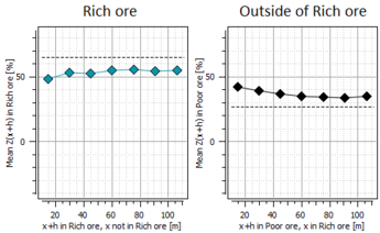
  • In the example below, we can observe that there are little border effects within ’Rich ore’ (left). The mean grade difference between ’Rich ore’ and its outside is essentially due to border effects outside ’Rich ore’ (right).

    Note: The horizontal line gives the mean grade of all data in the domain for x+h.

    

• Mean Difference [Z(x+h)-Z(x)]

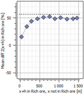
  • The mean difference [Z(x+h)-Z(x)] “across” borders of a domain A (i.e. when entering A) - samples at x+h being inside A and samples at x being outside A - can be visualized as a function of distance h (graphics displayed on the upper-left/lower-right diagonal):

    

  • The mean difference [Z(x+h)-Z(x)] between a domain A and a domain B - samples at x+h being inside A and samples at x being inside B - can be visualized as a function of distance h as (graphics displayed out of the diagonal):

    

  • In the example below, we can observe how the grade increases from outside ’Rich ore’ to inside this domain.

    

• Check Along assay trajectory to restrict the variogram calculations to samples belonging to the same drillhole only. This option is only available if the input data table is a drillhole file and is OFF by default.

• Display:

  • Check Mean difference to display the mean difference curves. By default, the program automatically calculates the graphic bounds accordingly to the data (based on the vertical minimum and maximum values for all the curves). However, you can specify new graphic bounds by entering values for Vertical axis min and Vertical axis max.
  • Check Global mean to add on all graphics the statistical mean represented as a dashed horizontal line.
  • Tick Number of pairs to display the number of pairs involved in the determination of each point of the variogram/covariance curves (for each lag). The display is possible as text or as histogram using the selector.
• Indicators per domain can be saved under a macro selection variable (for each index representing one input domain, the variable is equal to 1 if the grade variable belongs to the defined domain, and 0 if the variable is not in the domain) by checking the Save partial grade option. A default pattern Partial_%var helps you defining the output name.

Note: Samples that are not part of any domain are ignored.

H-Scatter

The H-Scatter plot item is meant to analyze the spatial continuity of the variable of interest.

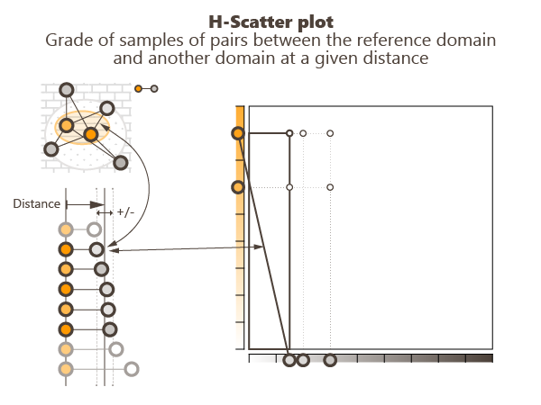
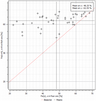
In the univariate case, this functionality allows the plotting of a scatter plot between the Grade variable and itself, that is the representation of all the pairs of samples whose locations are separated by a given vector. This vector is specified by its orientation and its elongation with a tolerance on both criteria. The coordinates along the X-axis and Y-axis are the two values of the variable at these two sample locations (see example below).

Note: The H-scatter plot is also available in the Exploratory Data Analysis, and can handle the bivariate case. However, domains are not used.

• Orientation: The H-Scatter Plot is a scatter diagram between the selected variable and itself. Each point on the graphic corresponds to a pair of samples such as their distance and orientation satisfy some constraints. These constraints are defined by:

  • the Distanceh and the associated tolerance t around this distance (+/-). Points of a pair separated by a distance whose value is included in this interval [h-t ; h+t] will be taken into account in the calculations.
  • the Rotation (for directional H-Scatter plot), given from an azimuth (N°0 pointing to the North) and a plunge (90° pointing down), to set the direction along which the pairs of points will be selected. A vertical direction is set by default. A tolerance is associated with the rotation. A pair of points will be taken into account in the calculations only if the angle between its orientation and the direction (on each side of the reference direction) is smaller than the tolerance.
  • the Radius (for directional H-Scatter plot), given by a length. It represents a cylinder lined up to the reference direction, out of which the pairs of points are selected (as for the variogram). The value you enter in the Radius box corresponds to the radius of the cylinder.

• Display

  The program draws a point each time the two variables are informed. Some other curves are also calculated by default:

  • the Mean Lines, called ’Means’ in the legend, which plot the mean on each axis and show the gravity center of the graphic. The mean values are printed in the view label and in the description of the reported graphic.
  • the First Bisector Line, called ’Bissector’ in the legend. This line is useful to analyze where a variable differs.