Special Options

• Special Options
  • Collocated Cokriging
  • Rescaled Cokriging
  • Filtering Model Components
  • Use Local Anisotropies
  • Use Uncertain Data
  • Take Faults into account
  • Reset negative weights to zero
  • Use customized output selection

This page depends on the options selected on the previous page.

Collocated Cokriging

Collocated Cokriging/Cosimulations is a particular case of cokriging/cosimulations a main variable using one or several auxiliary variables densely sampled.

The auxiliary variables are supposed to be known everywhere, i.e. at the input file sample locations and at the output file sample locations.

However the estimation at a given output file sample location makes only use of the values of the auxiliary variables collocated at this point and at the input file samples selected in the neighborhood search.

This method requires that a multivariate model be fitted to the main and auxiliary data variables, it should therefore have been specified in the Geostatistical Set.

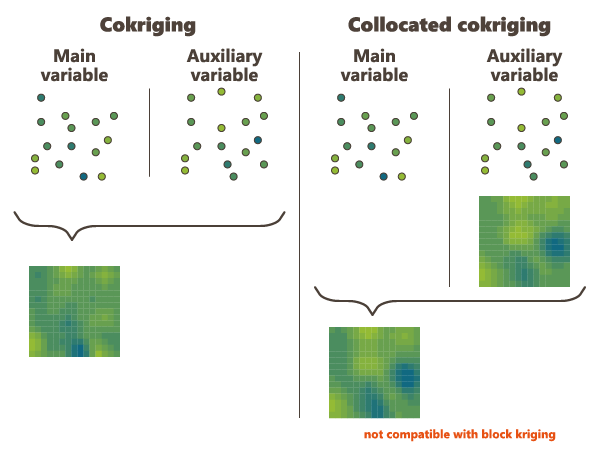
In general Collocated Cokriging is less precise than a full cokriging (making use of the auxiliary variable at all the output file sample locations when estimating each of these). Exceptions are models where the cross variogram (or covariance) between 2 variables is proportional to the variogram (or covariance) of the auxiliary variables. In this case collocated cokriging coincides with full cokriging but is also strictly equivalent to the simple method consisting in kriging the residual of the linear regression of the main variable on the auxiliary variable.

Note:If these variables are not consistent, the unbiasedness condition of Kriging no longer holds and the estimation results are unpredictable.

The Collocated Cokriging parameters are required if the Collocated Cokriging or Cosimulations Special Option has been chosen in the previous page. The objective is to inform the auxiliary variable(s) to be used for Collocated Cokriging/Cosimulations. The collocated variable(s) must match with one or several of the input data variables. It corresponds to the auxiliary variable which is defined simultaneously at the sample locations and at the target locations.

The collocated variable(s) can be located on the same output grid as the variable of interest. In this way, choose the Only Output Grid mode. Or the collocated variable(s) can be located on a different grid. In this way, choose the Only Auxiliary Grid mode and define the Data Table and an optional Selection on which the collocated variable(s) are. Then use the different selectors to indicate which collocated variable corresponds to each input variable. The variable of interest must be stay empty. If the Only Auxiliary Grid mode has been chosen, the collocated variable(s) will be interpolated on the final output grid using a bilinear interpolation.

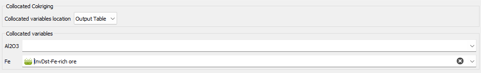
Note: Although this variable is defined in the output file, it is used as input information for Collocated Cokriging. Therefore, it must have values at target locations - no target points where the Collocated Variable is undefined will be estimated.

Rescaled Cokriging

Rescaled Ordinary Cokriging (sometimes referred as "Standardized ordinary kriging", SOCK) is a method that aims at reducing the risk of negative estimates because of negative weights assigned by Ordinary Cokriging to the secondary variables. The rescaled cokriging system replaces for n variables the n universality conditions required for unbiasedness by a single condition: the sum of all weights of all variables is equal to 1. Under the single universality condition the rescaled cokriging estimate is unbiased after having rescaled the secondary variables so that their means are equal to that of the primary variable. Consequently the values of the means of all variables must be known. Practically the means are provided exactly in the same way as for Simple Kriging (i.e. by checking the Strict stationarity option available in the Context section of the Variogram calculation in the Exploratory Data Analysis task). This option may be chosen when cokriging at least two variables.

The option is only available when a multivariate model has been fitted and strict stationarity has been specified in the input geostatistical set.

Note: This method was implemented from the following source: P. Ordinary cokriging revisited. Math. Geol. 30, 21, 1998. Goovaerts.

This method does not require any additional parameter than the means provided in the Geostatistical set.

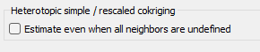
By default, if all the neighbors for one variable are undefined (heterotopic case), the estimated value is set to undefined. However, the equations can be solved even when there are no samples of the main variable and a special option is available to treat this case.

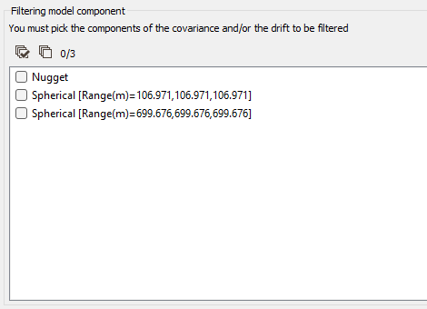
Filtering Model Components

If the model is made of several nested basic structures, you may consider that the phenomenon is a combination of several components - at different scales - which could be filtered out during the Kriging process.

By filtering out the appropriate components of the covariance part in the model, you can then estimate only the short range - high frequency - components or the long range - low frequency - components, instead of the entire phenomenon.

Moreover, this option also allows filtering out components of the drift part of the model.

Note: Filtering the Universality drift term consists in removing the contribution of the mean (either local or global depending on your Neighborhood choice). Similarly, filtering the X and Y Drift consists in removing the linear trend.

When activating the Filtering Model Components option, you have then to highlight the components of the Covariance and / or the Drift to be filtered from the model by ticking the corresponding structure(s) in the list.

Use Local Anisotropies

Local GeoStatistics is an original methodology fully dedicated to the local optimization of parameters involved in variogram-based models ensuring a better adequacy between the geostatistical model and the data.

It is used to determine and take into account locally varying parameters to address non stationarity and local anisotropies and allows to focus on local particularities.

The Local Anisotropies page allows to load the parameters required to perform Local Geostatistics (LGS).

The option requires a Grid data table on output. Variables corresponding to local parameters will be defined on the Output table or on an Auxiliary grid. They should have been previously created using Local Anisotropies functionality for example. Then you have to assign its variables to the corresponding moving parameters. You can define an optional Selection on the auxiliary grid.

Note: When choosing the Auxiliary grid mode, the local parameter will be interpolated at the target node locations. When using local rotation for neighborhoods or model, it is advised to check the output.

• Variogram model parameters (for all structures):

  • Select Rotation if you wish to make the model rotation varying locally. This option has a sense only if the defined geostatistical set contains an anisotropic variogram model.

    If your input data are 3D, select 2D (horizontal) to force and define a 2D rotation. Otherwise, choose the 3D option if you wish to define a 3D rotation.

    Select the Rotation variable that refers to the local rotation(s) in the local grid. To appear in the list, the variable should be associated to a Angle unit class in 2D and defined as a Rotation in 3D (see the Data Management / Create Rotation task). Be careful that the rotation is defined in the right Rotation convention.

  • Select Range factor if you wish make the different structure ranges varying locally. The ranges of the different structures will be multiplied by a given factor. This option has a sense only if the defined geostatistical set contains an anisotropic variogram model. The factor can be Global, in this way the proportion between all the ranges will be kept, or Per direction, to apply a factor different for each U/V(/W) direction.
  • Select Sill factor if you wish to make the sill varying locally. The sills of the different structures will be multiplied by a given factor (in this way each structure will be modified proportionally to the global sill). This option has a sense only if the defined geostatistical set contains a multi-structure variogram model.

• Moving neighborhood parameters: This section is designed to define local parameters for the Neighborhood. By default, same local parameters are defined for the variogram model and for the neighborhood. Click to unlock the link and to define different parameters.

  • Select Rotation if you wish to make the neighborhood rotation varying locally.

    If your input data are 3D, select 2D (horizontal) to force and define a 2D rotation. Otherwise, choose the 3D option if you wish to define a 3D rotation.

    Select the Rotation variable that refers to the local rotation(s) in the local grid. To appear in the list, the variable should be associated to a Angle unit class in 2D and defined as a Rotation in 3D (see the Data Management / Create Rotation task). Be careful that the rotation is defined in the right Rotation convention.

  • Select Ellipse radius factor if you wish to make the neighborhood radius varying locally. The factor can be Global, in this way the proportion between all the radius will be kept, or Per direction, to apply a factor different for each U/V(/W) direction.

Note: All the variables defined in this panel are read from the local grid. The local grid must be of the same dimension (2D/3D) as the input data file it is referring to.

Use Uncertain Data

This option enables taking into account uncertainties associated to the input data points: either giving standard deviation measurement errors at data points in addition of the data value or providing only an interval of the data value (the exact value is unknown but we can define a lower and/or an upper bound value) (only available in the Kriging task).

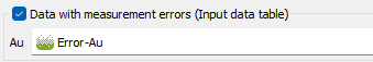
• Data with measurement errors (Input data table): this option is based on a Kriging with Variance of Measurement Error (KVME). Be careful that here, in Isatis.neo, we ask for a standard deviation (with the same unit class as the input data) and not a variance.The method can be applied if one of the data variables - defined on the input file - could be considered as polluted by some particular type of noise, with the following properties:

  • This noise cannot be considered as constant all over the field area - otherwise it could be modeled with a standard nugget effect in the model - Instead it is defined by its standard deviation at each sample location which will be used in the kriging system.
  • It has not been taken into account while fitting a model on the data variable. The structural analysis must have been achieved on a clean subset of the polluted variable.

  Choosing this option, you have to specify one or several variable that contains the amount of noise, i.e. the standard deviation, at each sample location (defined on the input Data Table).

  

Take Faults into account

The faults are defined as portions of the space which can interrupt the continuity of a variable. They are introduced here to take into account geographical discontinuities in kriging interpolation (i.e. during the conditioning step). Basically, faults are used as "screens" when searching for neighbors during estimation. A sample will not be used as neighboring data if the segment joining it to the target intersects a fault.

We consider two kinds of faults:

• 2D faults which are defined as polylines (vertical faults and/or polygonal faults for faults with dip). These faults can be imported through the Vector File Import that gives you the choice of output (polygons or polylines). Polygons will be read as closed polylines in this case. With 3D data, faults will be considered as the projection of a vertical wall.

  This option requires to provide the faults file (i.e. a polyline file) and an optional selection if you want to consider only a subset of your faults file. Three calculation modes are offered (only when working with 2D datasets):

  

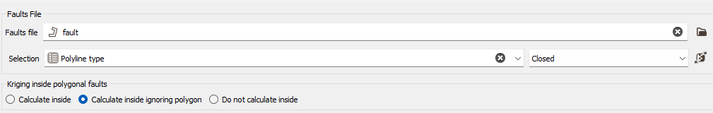
  • Calculate inside: the data used in the kriging process to estimate a node inside the polygon will belong to this polygon only,
  • Calculate inside ignoring Polygon: the polygonal fault will be considered as transparent for the estimation of the nodes inside the polygon,
  • Do not Calculate inside: no node value will be calculated, it will be put to undefined. This allows you to consider for instance this polygonal fault as a crushed zone where no estimation is realistic or a different estimation method has to be used.

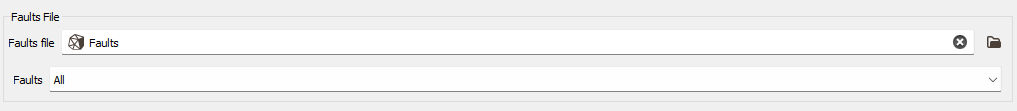
• 3D faults which must be defined as meshes. In this case no option is required, except the definition of the faults file and an optional selection if you want to consider only a subset of your faults file.

  

Reset negative weights to zero

The aim of this option consists in resetting negative weights values to zero in Ordinary Kriging and Simple Kriging. Modifying the weights generally avoids getting values outside the original range of values (greater than the minimum input value and smaller than the maximum input value).

Negative weights are set to zero. If the sum of weights is greater than one, then the weights are rescaled so that they sum to one. In the Ordinary Kriging case, this will always lead to rescaling (because the sum of weights started at one, and the elimination of negative weights makes the sum greater than one). In the Simple Kriging case, this may or may not lead to a rescaling.

Use customized output selection

Define a selection variable (or a categorical variable or a macro-selection) that will be used to apply the cross-validation on a subset of the data defined by the input geostatistical set .

Note the difference between the selection defined by the geostatistical set and the customized output selection applied to the data. The customized output selection provides the set of target points on which the cross-validation will be carried on, whereas the selection defined by the geostatistical set gives the set of active data points that might be used for this test.