
Variogram Model
These parameters allow you to fit a model on the experimental variogram(s). Modeling consists in finding a single mathematical function which will capture the spatial behavior of all the variables for all the directions of the space. The model will be saved in the Geostatistical Set and used for subsequent Kriging / Simulations process.
The model is obtained as a linear combination of basic structures, characterized by their type and range. The weights in this linear combination correspond to the sills. In the multivariate case, the set of all the sills constitute the coregionalization matrix for each basic structure.
The principle is to minimize the distance between the model and all the different experimental variograms for any calculation distance.
Interface
-
Click Load Parameters to initialize the new model from an existing one (saved in a Geostatistical Set) and select the Geostatistical Set of your choice. Be careful this variogram must have been calculated on the same type of data to be consistent.
All the variogram model parameters (structures, sills, ranges, rotation...) will be reloaded. If the chosen Geostatistical Set contains both a raw and a gaussian model, then both will be loaded (if both have been calculated). Then go to the Fitting window to improve the model.
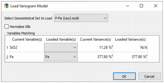
In case of a multivariate Geostatistical Set, a matching table is presented to define to which current variable you want to associate the loaded model. Each corresponding variance is displayed for information. A Normalize Sills toggle can be activated to rescale the global model variance to the variable variance. This option is set by default.
Note: Old Geostatistical Sets (prior to the 2020.10 version) cannot be reloaded. They are greyed out and identified by an (Obsolete) suffix.
- Tick/untick the Model Fitting option to display or not the variogram model.
-
If the Model Option in the Context section is Compute Raw Model Only or Compute Gaussian Model Only, a single Fitting button will be reachable. However if the Model Option is Compute Raw & Gaussian Model, a selector appears with two choices:
-
Deduce the Raw Model from Gaussian Model: in this case, you will access the gaussian model fitting parameters and the raw model will be deduced from the gaussian one. An automatic fitting will be done using the same set of input structures (ranges and sills proportions will not be kept, only the selected structures).
Note: This calculation mode is not available when having a Zero effect applied on the Gaussian variable.
- Fit the Gaussian and Raw Model Independently: in this case, you will access both gaussian and raw model fitting parameters through two dedicated buttons Gaussian Fitting and Raw Fitting.
-
Variogram Fitting
Two fitting buttons are available and open a new window: Raw fitting and Gaussian fitting.
-
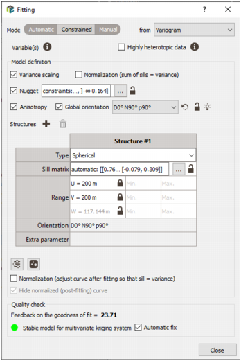
The Fitting utility offers three modes:
- The Automatic fitting procedure calculates optimal sills, ranges and anisotropies from any set of basic structures.
- The Constrained fitting procedure calculates the optimal parameters (sills, range values, anisotropy), once some other model parameters have been specified.
- The Manual fitting procedure lets you define all the parameters and values of the model. In batch, when using this mode, the model to be created will have the same parameter values as the ones that you are about to create.
-
Fitting from: Select the curve type on which you want to base your fitting. It can be any curve (covariance, madogram, etc), except the cross over simple variogram.
Note: If the Zero effect is applied on the anamorphosis, only the variogram and covariance can be used here.
However, sills are always shown in the fitting window as variogram or covariance sills, even if the model has been fitted to one of the other curves. To draw a model curve over one of the other curves, the sills are suitably scaled. The scale is to 1 for correlogram, and to an estimated sill (by random sampling) for pairwise-relative variogram and madogram.
You can tick the Variance scaling option in order to have parameters expressed as a ratio of the variance.
-
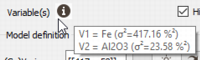
Variable(s): The objective of this information area is to recall variable properties (names and variances). This is particularly useful in multivariate to know which variable is V1, V2, etc, in the nugget and sills matrices (the order of the different variables depends on the selection order in the variables list).
-
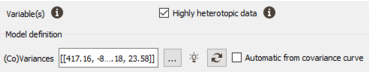
The option ’Highly heterotopic data’ is displayed in multivariate cases with omnidirectional or multidirectional calculations only (not in downhole). To help you in the decision, a tooltip explains the heterotopic situation.

If the Highly heterotopic case is selected, then a new section Define covariance at origin appears. By default, if a pair of variables has less than 10% of defined samples at the same location, the option is activated. The goal is to enable the user to set the values of the simple and cross-covariances at a 0-distance (particularly in the heterotopic case, for which the origin of the function could be poorly defined). Indeed, the values of C00 can be experimentally calculated only for the points where the variables are simultaneously defined. In the true heterotopic case, the cross-covariance at 0-distance is not even defined because there is no point where the variables are simultaneously defined.
The option ’Automatic from covariance curve’ means that the automatic value for C00 is defined after the experimental variogram calculation.
The matrix is the covariance at origin matrix for the variables. It is symmetric and the diagonal corresponds to the variances. It can be edited by the user. In case of an impossible system (i.e., there is at least one negative eigenvalue), a message is printed and the matrix must be fixed using the ’Fix’ button on the bottom of the window.

In the Covariance and Correlogram curve types, the C00 value is displayed as a black cross on the graphics, and the C00 values are written in the view label.

-
The Variance scaling option enables you to define and display the variogram model as a proportion of the variance (i.e. between 0 and 1 for simple variograms, -1 and 1 for cross-variograms, and without unit). The sill of each structure, as well as the nugget, is divided by C00. This option is only available for the raw models (not the gaussian ones).
The Variance scaling state is saved in the Geostatistical set information. It is used as the default state when printing, editing and displaying the raw model from the Geostatistical set explorer.
-
The Normalization option enables you to normalize the sill of the simple variograms to the experimental variances (1 in gaussian) or to the correlations for the cross-variograms. Two modes are available:
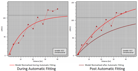
- Normalization (sum of sills = variance): This normalization is performed during the automatic fitting procedure. It automatically adjusts the experimental curve by honoring the experimental variance (the sum of the sills will be equal to the variance). This option is disabled in manual fitting mode.
- Normalization (adjust curve after fitting so that sill = variance): This normalization is performed at the end of the fitting procedure as a post-processing. It automatically adjusts the experimental curve and rescale after the sills to the experimental variance. When choosing this option, the normalized curve is also displayed by default in addition to the "original" curve. Activate the Hide normalized (post-fitting) curve to only display the original curve (the curve which corresponds to the entered parameters).
This option is not compatible with non stationary structures (as linear structure for example).
Note: The normalization to 1 is performed for the Gaussian case, for which the variance should equal 1.
-
Tick the Nugget toggle to add a nugget effect in your model.
- In Automatic mode, the value of the fitted nugget effect is displayed for information.
-
In Constrained mode, you can lock a given value. In this case, a
 icon is displayed. Alternatively, you can enter a Minimum and/or a Maximum value. The minimum and maximum are both inclusive. Leave the values empty to ignore the minimum or maximum value. These values are expressed in the variable squared unit or are between 0 and 1 if the Variance scaling option has been chosen.
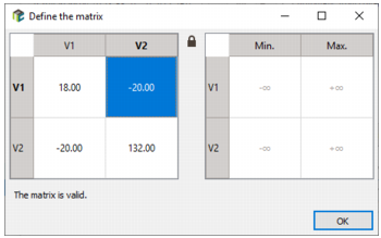
- In Manual mode, enter the value of the nugget effect you want to consider for your model. This value is expressed in the variable squared unit or is between 0 and 1 if the Variance scaling option has been chosen.
In multivariate, a button ... appears to access the matrix of the nugget effect for the whole set of variables, the diagonal being the nugget effects defined for each simple variogram. This matrix refers to variables called V1, V2, ... The Variable(s)
 button allows verifying to which real variable name the Vi naming corresponds. In constrained mode, you can either define given values for the full matrix or an interval (with a minimum and/or a maximum) for the diagonal but the two options cannot be mixed (i.e. the first variable associated to a given value and the second variable constrained to an interval).
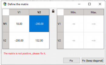
The matrix of nugget effects is symmetric and must be positive semi-definite (its eigen values are all non-negative). When modifying a value of the matrix, you have to check its validity before applying the modifications. If the matrix is not positive semi-definite, an error message is printed at the bottom of the interface and the modifications are not accepted. Click on:
- Fix to obtain a positive semi-definite matrix by decomposing the matrix with eigenvalues and eigenvectors, setting negative eigen values to 0 and rebuilding the original matrix. Unfortunately, this direct correction does not guarantee that the diagonal terms are preserved.
-
Fix (Keep Diagonal) to obtain a positive semi-definite matrix keeping the values on the diagonal unchanged. This second procedure is proposed as an alternative option. This iterative procedure has the advantage preserving the diagonal terms.
-
Check the Anisotropy option to model a variogram with an anisotropy. Note that this feature is only available when a multidirectional experimental variogram has been calculated and is active by default in this case. This gives access to the Global orientation option which forces the rotation to be global over the structures. This means all the structures will have the same rotation. The value of the global orientation is set by default to the same reference orientation defined for the experimental curve.
- In Automatic mode, the global rotation is displayed for information.
- In Constrained mode, the global rotation can be edited and modified. To lock this parameter for the fitting, enter the value you wish to use and click on
 . This value will be stored in the batch file. If you don’t want to use the lock value option, leave it off. In this case, the value stored in the batch file will be set to automatic.
 -
In Manual mode, the global rotation can be edited and modified. This value is used for the fitting and will be stored in the batch file.
Note: The angles used for the rotation definition are explained in the Rotations section of the online help.
-
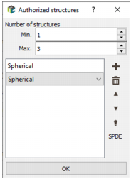
Click on Authorized structures to select the structures on which you want to base your Automatic fitting. Click
 to initialize the structures with the ones defined by the Setting up Preferences. By default in Isatis.neo, this is a cubic, an exponential, a spherical and a linear, plus a nugget effect (the default structures can be different in the Mining and Petroleum versions). The SPDE button allows the use of structures compatible with the SPDE methodology (i.e. Matern structures). The order of the defined structures is important. It is recommended to initialize the structures by increasing continuity (for example, enter a cubic, then an exponential and a spherical).
These are the most common sets of structures. If the Normalization option has been checked previously, non stationary structures will not be available. If you want to use other structures, play with the
 and
and  to add / remove structures. The order of the defined structures also influences the result of the fitting. Use the arrows to modify the order of the selected structures. The Automatic Fitting procedure can discard a given structure, if this given structure does not improve the fitting. To avoid that, you can set a Minimum / Maximum Number of structures. This enables you to enter a smaller / bigger number of structures but keeping only a reasonable number of them.
-
When using the Constrained or the Manual fitting mode, the panel allows you to define all the parameters and values of the model. Click
and to add / remove structures. For each selected structure, define its type, sill(s) and range(s). - When deactivating the Anisotropy toggle, the ranges along the different directions U, V and W will be linked with a same unique value.
- If you have not chosen a Global orientation, you can also define an orientation per structure.
-
In Constrained mode, you can either lock a given value (a full sill matrix and/or a range) by clicking on . Or you can enter a Minimum and/or a Maximum value (only for ranges). Both options can be mixed for ranges. The minimum and maximum are both inclusive. Leave the values empty to ignore the minimum and/or maximum value. These values are expressed in the variable squared unit or are between 0 and 1 if the Variance scaling option has been chosen. When a parameter is locked , the corresponding value will be stored in the batch file. When the lock value option is off, the value stored in the batch file will be set to automatic.
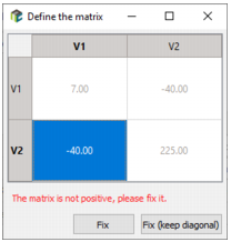
In multivariate mode, a button ... appears to access the sill matrix of each structure, the diagonal being the sills defined for each simple variogram. This matrix refers to variables called V1, V2, ... The Variable(s)
button allows to verify to which real variable name the Vi naming corresponds.
-
The matrix of sills is symmetric and must be positive definite (its eigen values are all strictly positive). When modifying a value of the matrix, you have to check its validity before applying the modifications. If the matrix is not positive definite, an error message is printed at the bottom of the interface and the modifications are not accepted. Click on:
- Fix to obtain a positive definite matrix by decomposing the matrix with eigenvalues and eigenvectors, setting negative eigen values to 0 and rebuilding the original matrix. Unfortunately, this direct correction does not guarantee that the diagonal terms are preserved.
-
Fix (Keep Diagonal) to obtain a positive definite matrix keeping the values on the diagonal unchanged. This second procedure is proposed as an alternative option. This iterative procedure has the advantage to preserve the diagonal terms.
-
Click
 to access the Advanced fitting parameters. The automatic fitting algorithm is made to minimize the distance between the model and all the different experimental variograms for any calculation distance. The automatic fitting procedure helps you adjust the model by calculating optimal sills, ranges and anisotropies from any set of basic structures. We define a Maximum number of iterations to test to meet the minimization criterion. If the criterion is not satisfied, an error message to say that the algorithm failed the fitting will be printed. The Reject structure criterion and the Reject nugget criterion respectively represent the percentage of variance below which a structure and the nugget effect will be discarded.
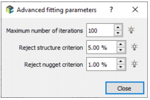
-
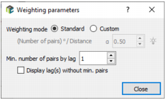
Click
 to access the Weighting parameters. The principle of the Automatic fitting procedure is to minimize the difference between the experimental value of a variogram lag and the corresponding value of the model, and to repeat this operation for all the variogram points. This minimization is carried on giving different weights to the different lags. The default weights, defined by the Standard mode, are computed using the following formula:

Choose the Custom mode to access and modify the power of the ratio between the number of pairs and the lag. This α parameter is a float value lying between 0.1 and 2. A small value should increase the weight of the lags corresponding to the smaller distances.
Enter a value for the Min. number of pairs by lag. This option enables you to automatically discard all variogram points where the number of pairs is too small.
Tick/untick the Display lag(s) without min. pairs option to display or not the lags which have been removed from the automatic fitting because they do not have enough pairs of samples.
-
Display upscaled curve with Zero effect: This option is only available in the Gaussian fitting window, when the Zero effect is applied on the anamorphosis.
The experimental variogram is calculated from the truncated Gaussian variable (taking into account the zero values). The model is adjusted on the experimental curve. However, the numerical parameters of the model are based on the final variogram. Hence, it is possible to display this final upscaled variogram. It appears on the graphic with a lighter color. For further estimation / simulation, the upscaled variogram will be used. The default of this option is OFF.
-
Quality check:
-
A Feedback on the goodness of fitting (GOF) is printed to check the adequacy between the experimental data and the fitted model (for the fitted curve and for the variogram if they are different).
The GOF is a weighted sum of the difference between the model evaluation and the experimental values at the experimental lags:

The GOF is an error measurement to minimize but its intrinsic value cannot be interpreted as it to infer on the adequacy between model and data. It should be used to compare different models fitted on the same experimental data (with the same experimental parameters) and to see if one is better than the others.
-
A check is done on multivariate variogram models to protect from numerical instabilities while kriging. This kind of problem can happen when the cross-variogram model is very close to perfect correlation between the variables.
For each structure of the cross-variogram model, including the nugget, we create a simple cokriging system and we test for each variable if any of the weights are suspiciously large.
A feedback on the presumed stability of the multivariate model is displayed in the interface. Green, when everything is ok. Orange, when we suspect the model to be unstable. In this case, check the Automatic fix toggle in Automatic and Constrained modes or click on the Fix button in Manual mode to automatically modify the model. A correction is applied on the sill matrices in order to make it stable (we reduce by 2% the off-diagonal terms of one of the structures). This option is offered in the Automatic and Constrained modes to be registered and applied when saving/running the batch. If the automatic fix has been applied, a feedback ‘(Fixed)’ is printed on the right of the option.
-
Note: Variogram can also be fitted interactively activating the Interactive Fitting Mode in the Graphical Options.