Linear Interpolation
The Linear Interpolation is meant to estimate variables from gridded data to an output dataset of any geometry type.
Another particular aspect of Linear Interpolation is that it enables interpolating two categories of variable: standard numerical variables and rotations, a specifically designed interpolation algorithm being applied for rotations.
To summarize, the linear interpolation mainly consists, for each output target point, in evaluating weights for the input gridded data surrounding the target point. Then, the output variables are estimated from a linear combination of the input data using these weights. For standard numerical variables, several interpolation options are proposed to configure this process.
Parameters
-
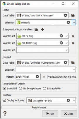
Input:
- Data Table: The input data set is the grid data table containing the variable to estimate, which must already exist. Click the directory icon
 next to Data Table to open a Data Selector and select the data table on which the Linear Interpolation task will be applied. The Data Table can also be dragged and dropped directly from the Data tab.
 - Selection: A selection can also be provided to use a specific subset of the input data for the interpolation.
-
Interpolation input variables: The variables to be interpolated can be selected within the following choices:
- Numerical,
- Rotation 2D: for angle variables,
- Rotation 3D: for 3D rotation compound variables.
Click
 to add another variable in the list and
  to remove a variable from the input list.
Note: The Create Rotation Compound Variable task, accessible from Data Management / Create Compound Variable / Rotation, can be used to generate the rotation compound variable from the 3 unit rotations components and the wanted rotation convention. It only requires checking the Initialize Components From Existing Angle Variables option.
Note: For rotation variables, the Interpolation Option is forced to Standard. The rotation interpolation is based on the quaternions method.
- Data Table: The input data set is the grid data table containing the variable to estimate, which must already exist. Click the directory icon
-
Output:
- The Output dataset, onto which the input variable(s) is/are interpolated, can be of any geometry type, unlike the input data set. It must already exist.
- Selection: A Selection can also be provided to perform the estimation on a subset of the output dataset.
-
Pattern: In the Pattern field, a customizable generic name is proposed to automatically generate the output variable names. By this way, if the estimation process is applied on several input variables, it is not necessary to manually enter the output name for every variable. A preview shows the resulting output name for the first selected input variable.
Note: If the Linear Interpolation is applied on several variables, the pattern must contain the %var keyword. Then, %var will be replaced by the input variable name, e.g., if the input variable is called V1, %var-LinearInterpol will lead to the output name V1-LinearInterpol.
-
Interpolation Option: Furthermore, for Numerical variables, an Interpolation Option is then proposed with the following choices:
- Standard: if an output target point is outside but sufficiently close to the input data field, the estimation is performed.
- No Extrapolation: if an output target point is outside the input data field, the estimation is not performed and it will be set to undefined.
- Extrapolation: the estimation is performed even if the output target point is far from the input data field.
To finish, the output variables can be displayed in the 3D Scene or Map, respectively for 3D and 2D data, by checking the Display in Scene option and selecting the wanted scene.
Results
As output to the estimation process, the output variables whose names have been generated from the pattern are saved into the output data set. If the Display in Scene option has been selected, they are displayed in the chosen viewer. The option is compatible with numerical variables and rotations.
Note: The 3D viewer allows editing aspects of displayed variables from Layer Properties. For instance, rotations can be displayed as an RGB system, each color corresponding to the U, V, W axes after the rotation application. The axes to display can be selected in the Vector menu.
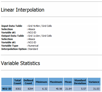
In addition, a summary is displayed in the Messages Window to recall the entered parameters, i.e. the input and output data tables with their respective selections, the input and output variables, the variable type and finally the interpolation option. Some statistics on the output variables are also displayed: total count, defined count, minimum, maximum, mean, standard deviation and variance.