MIK Post-processing

The purpose of this tool is to calculate quantities - such as an e-type estimate or grade-tonnage variables - based on a series of indicator estimates.

Preliminary steps

Note: The use of the MIK Post-processing task should follow the variogram modeling and the kriging steps.

In the Exploratory Data Analysis, you should create one raw variogram per indicator. When saving the variogram, a message is printed telling that the geostatistical set will be saved in the vendor data information associated to the MIK macro variable.

Then, the different variograms will be used in the kriging. In input, select one of the geostatistical sets done on the indicators. Activate the Multiple kriging special option.

Note: The Multiple kriging option is not compatible with all the other ones.

The next page is dedicated to the Multiple kriging entries. It consists in having the list of all the indicator values (read from the macro variable of indicators) and matching a geostatistical set to each selected one.

The same neighborhood will be used to krige all the indicators. Note that the capping is not available.

The Run will loop over the different geostatistical sets, and will create one macro variable in the output data table, with one kriged indicator per index. The statistics of the kriged indicators are printed in the Messages window.

Main interface

The interface of the MIK Post-processing task is divided into two columns: on the left are the inputs and the local histogram interpolation parameters, on the right are the outputs and the volume correction parameters.

Input

Data table: The data table (usually a grid) containing the estimates of the indicators.
Selection (optional): If set, the calculations will only be performed on blocks or samples inside the selection.
Filling-in mode: other fields will change according to the chosen mode.
- Kriging macro variable: use this mode when having one macro variable in output from the kriging (thus, using the Multiple kriging option). The linked vendor data should already get all the needed information to fill in the inputs.
  - Kriging macro variable: This is the macro variable containing the kriged indicators, likely created by the kriging task. It is used to read the indicator values, which are written in the indices of the macro variable, and associate one kriged indicator to one indicator value. The table below should be automatically populated.
- Several kriging variables: use this mode when having several variables in output of the kriging (not using the Multiple kriging option).
  - Macro variable indicators: The macro variable containing the indicator values, likely created by the MIK Pre-processing task.
  - Variable pattern: A pattern to describe the names of the Kriged indicators. The table below this pattern shows the list of indicator values (read from the Macro variable indicators) and allows you to choose the variable in the Kriged Data Table containing each indicator's estimate. If you set the pattern to match the naming convention of the variables (e.g. "%var_#%indicator", or "OK-%var_#%indicator-Krig"), then clicking the magic wand in the 'Variable' cell will automatically populate the table with the estimated variable names.
Indicator table:
- When using the Kriging macro variable mode, the table is entirely read-only because it should have been filled in correctly from the vendor data of the Kriging macro variable.
- When using the Several kriging variables mode, only the indicator values are filled in. You need to associated one kriged variable per indicator, the pattern (as explained above) can automate the research.

To remove an indicator value and its associated kriging result from the post-processing calculation, untick the checkbox of the adequate line in the indicator table.

Note: When using the Class mean method (explained below), a column Mean is added to get the mean value among the class. These values are editable.

Method

Histogram interpolation: the kriged indicators are interpolated and extrapolated to make a model of the full cumulative distribution function (CDF).
Class mean: a mean value is assigned to each indicator interval class, and these are used to calculate the e-type estimate.
- The mean of each class is printed and editable in the Indicator table above. There is one mean per indicator value. The mean above the last indicator is written in the following dedicated field.
- The automatic values are calculated in the MIK pre-processing task (and stored in the vendor data). Commonly, the input data mean is used for each class except the upper tail, for which the input data median is used.

Note: The class mean method allows you to calculate only the mean and error outputs, because the full CDF is not known.

Local histogram interpolation parameters

Note: These parameters are already proposed at the MIK Pre-processing step, with an additional graphic to visually see the impact of the parameters. Here, they are automatically set from the parameters used in the MIK Pre-processing step.

The Kriged indicators only give a relatively small number of points in the local (complementary) cumulative distribution function. To calculate statistics, the full distribution is needed, and that requires interpolating between indicators, and extrapolating the tails. The parameter choices made here can have a substantial impact on the results, in particular for upper tail when the original data is highly right-skew.

The statistics printout from MIK Pre-processing in the Messages window gives some possible values for the exponents, but does not say if one model or another is a better fit to the data.

Note: These transformations of the indicator Kriging results have been inspired by the GSLIB methods and we strongly recommend the user to refer to the paragraph V.1.6 "Going Beyond a Discrete CDF" of the GSLIB User Guide (Deutsch and Journel - Oxford 1992) to understand the methodology and the corresponding parameters.

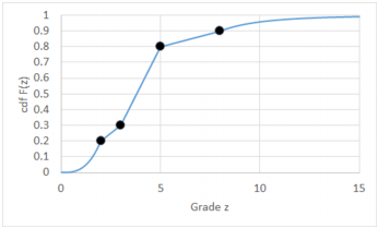
There are four types of interpolation models offered. In the following descriptions, z₁, z₂,…, z_n are the indicator thresholds, and F(z) is the cumulative distribution function, i.e., the probability to be less than or equal to z. The Kriged indicator for z_i is 1-F(z_i), and the formulas below describe the interpolation between consecutive thresholds z_i and z_i+1.

Linear model:

This is a linear (straight line) interpolation between points on the cdf, corresponding to a uniform distribution between z_i and z_i+1.
Power model:

The exponent α must be greater than zero.
- α < 1: Right-skew distribution between z_i and z_i+1.
- α = 1: Uniform distribution; identical to linear model interpolation.
- α > 1: Left-skew distribution.
Beta power model:

The exponent β must be greater than zero. This model is effectively a mirror-reversed version of the power model. When β>2, the modelled histogram will smoothly decay to zero at the upper bound of the interval.
- β < 1: Left-skew distribution between z_i and z_i+1.
- β = 1: Uniform distribution; identical to linear model interpolation.
- β > 1: Right-skew distribution between z_i and z_i+1.
Hyperbolic model: This model is only used for the extrapolation above the last indicator z_n (which must be positive), i.e., for the upper tail. Outside of geostatistics, it is usually known as the Pareto distribution.

Unlike the linear and power models, this distribution is unbounded, with the cdf only asymptoting to 1, never actually reaching that value. The exponent α controls how fast cdf approaches 1, or equivalently how long the tail is - a smaller value of α gives a longer tail and a higher mean (e-type estimate). The exponent must be greater than 1.
- 1 < ɑ ≤ 2: The mean of the distribution is finite, but the variance is theoretically infinite. (An output standard deviation variable will nevertheless be finite, because of the finite number of discretization steps used in the calculation.)
- α > 2: Both the mean and variance are finite.

Different interpolation choices can be made for three cases:

Lower tail interpolation: Choice of linear model, power model, and beta power model; extrapolation will be between the Minimum value allowed and the first indicator threshold. A power model is a common choice. The Minimum value allowed defaults to the first indicator threshold, and would usually be replaced by the minimum of the original variable.
Within-classes interpolation: Choice of linear model, power model and beta power model; this is the interpolation between indicator thresholds. The linear model is a common choice.
Upper tail interpolation: Choice of linear, power, beta power and hyperbolic models. In the case of the linear, power and beta power models, extrapolation is between the last indicator threshold and the Maximum value allowed, at which point the cdf reaches 1. For the hyperbolic model, which is unbounded, this maximum is ignored. The choice of model and exponent here is often the most critically important. Guessing exponents without studying the distribution of your original variable may lead to drastic over-estimation of the mean grades or metal quantity above a cutoff.

A hyperbolic model is common when the original variable is highly right-skew, i.e., there is a long tail of high values, as is often the case in gold.

A stylized graphical example of such interpolation is shown below, using only four indicators. A power model (exponent 3) is used between zero and the first indicator, a linear model is used between indicators, and a hyperbolic model (exponent 4) is used above the last indicator.

There are two choices for the Calculation method:

Exact: Theoretical values (integrals) from the model parameters will be used where possible, and the task will do a numerical computation to within a relative error Tolerance otherwise. The numerical computations are used when there is an indirect lognormal correction combined with:
- a power model with a non-zero lower bound of the interval; or
- a beta power model.
Discretization: The probability axis between 0 and 1 is discretized into a given number of Discretization steps. This parameter controls the precision of the calculations, which are integrals over the probability axis between 0 and 1. A larger number of discretization steps gives a more time-consuming and more precise calculation. If the number of steps is 100, then all output tonnage variables will have values that are an integer number of percent. If the number of steps is 1000, then the tonnages will be given to a precision of 0.1%.

Output

Variable pattern: The pattern to be used for the output variables, listed below.

Only the ticked following outputs will be calculated at the Run.

QTM: The tonnage variables, representing the quantity of metal Q, the tonnage T, and the mean grade M above entered cutoffs. The implicit assumption is that the probabilities defined by the Kriged indicators can be interpreted as proportions of a block.

The usual mining context for this calculation is that the indicators have been Kriged onto a panel grid, and that selection of blocks above grade cutoffs will be made at selective mining unit (SMU) scale, where the SMUs are smaller than the panels In such a case, it is appropriate to apply a volume correction for the change of support from points to SMUs; options for this correction will appear if the QTM output option is selected, along with a list of cutoffs.
Mean: The estimated value for the output location, commonly called the e-type estimate. It is the expectation of the distribution defined by the Kriged indicators and the histogram interpolation parameters.
Standard deviation: The standard deviation of this distribution.
Variance: The variance of the distribution.
Quantiles: Values at entered quantiles of the distribution; an option to choose the quantiles will appear if this output variable is selected.
Error: An error code variable, to flag if any adjustment to the Kriged indicators was made. Code values are as follows; the code values are added together if more than one type of error occurs.
- 0: No changes.
- 1: At least one Kriged indicator was less than zero, and was corrected to zero.
- 10: At least one Kriged indicator was greater than one, and was corrected to one.
- 100: At least one Kriged indicator is greater than the previous Kriged indicator. In this case, order relation corrections are applied in an identical fashion to the GSLIB procedure.
As an example, suppose that there are five Kriged indicators, with the grades in parentheses:

IK(1) = 0.46, IK(2) = 0.40, IK(3) = 0.33, IK(4) = 0.37, IK(5) = 0.21.

Here, the indicator at a grade of 4 is greater than the indicator at a grade of 3, a logical impossibility.

The correction is applied in three steps. Firstly, loop through the indicators from the lowest threshold (index) upwards. If a Kriged indicator is greater than the previous, then set that indicator to the previous value:

IK'(1) = 0.46, IK'(2) = 0.40, IK'(3) = 0.33, IK'(4) = 0.33, IK'(5) = 0.21.

Secondly, loop through the original indicators in reverse order. If a Kriged indicator is less than the next one, set that indicator to the next value:

IK''(1) = 0.46, IK''(2) = 0.40, IK''(3) = 0.37, IK''(4) = 0.37, IK''(5) = 0.21.

Finally, take an average of the two corrections to produce the final set of corrected indicators, IKcor(i) = 0.5*(IK'(i) + IK''(i)):

IKcor(1) = 0.46, IKcor(2) = 0.40, IKcor(3) = 0.35, IKcor(4) = 0.35, IKcor(5) = 0.21

Note: Only the Mean and Error outputs can be selected when using the Class mean method.

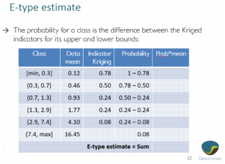
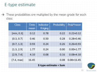
Details about the E-type estimate

The e-type estimate is calculated when using the Class mean method.

The three following images detail the calculation step by step.

Volume correction

The Volume correction option here is only shown if the QTM output variables are to be calculated. The assumption is that the ccdf from the Kriged indicators is a ccdf of a variable on point support, but that recoverable resources should be based on selections made at block support, where the block is the size of a selective mining unit. Since block values will be smoother than point values, it is appropriate to reduce the variance of the local ccdf before calculating tonnages above cutoffs.

The following section is here to help you defining the volume variance correction factor. It requires:

A variogram model, contained in the Geostatistical set of raw variable (i.e. the geostatistical set of the input grade variable). If not provided, the variability table will not be visible and the SMU and the input support information will be disabled.
A dimension of the SMUs, SMU block size, with a given SMU block discretization. The size of the SMU block must match the size of the input support (i.e. it must be a multiple of the input support size). By default, a discretization of (5, 5, 3) is set.
A panel block model with a given Input support discretization, (5, 5, 3) by default. The size of the panels is directly read from the input data table. In case where the input data table is not a grid or if there is no parent grid in case of sub-blocks, an additional Input support size has to be defined.

The variability table summarizes the different quantities:

Variogram sill:
Grade variability in SMUs:
Grade variability in input support:

Since the grade variability increases when the support size increases, we should have:
SMU variability in input support:
SMU block variance:
Input support variance:
Global variance correction factor:
Local variance correction factor:

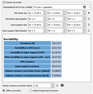
There are two options for how to perform the variance reduction, both of which use the Volume variance correction factor, denoted by f.

Affine correction: The distribution is squashed linearly towards the mean, preserving the overall shape of the distribution, except that it becomes narrower. (So, for example, the skewness remains unchanged.) If m is the mean of the local ccdf, and q a quantile, then the corrected quantile q_v for the blocks is:

See An Introduction to Applied Geostatistics, E.H. Isaaks & R.M. Srivastava, Oxford University Press, 1989, p 471. In this case, the minimum and maximum allowed values are also transformed towards the mean.
Indirect lognormal correction: Quantiles of the point ccdf are transformed assuming that both the point and block values are lognormally distributed; this has the effect of de-skewing the distribution, making it more symmetrical. See Isaaks & Srivastava (op cit.) pp 472-476.

The mean m and coefficient of variation CV are calculated from the ccdf. Then the quantiles are first transformed to:

where

and

When the ccdf is not precisely lognormal, this transformation can change the mean, to some value m'. To ensure consistency, the transformed quantiles are transformed a second time, by:

There remains the question of what the Volume variance correction factor should be. It is the ratio of the variance on block support to the variance on point support:

Given a variogram and Gaussian anamorphosis of the original variable, inputs to this calculation can be found from the statistics printed after running Support Correction (the "Point Variance (Anamorphosis)" and "Real Block Variance").

Cutoffs definition

This is only shown if the QTM output variables are to be calculated. The tonnages, metal quantities, and mean grades are calculated above the cutoffs defined here.

Click on to set default values for the lists.

Click Edit to pop up the Value Definition window and customize the list of cutoffs.

Quantiles definition

This is only shown if the Quantiles output variable is to be calculated. The chosen quantiles of the local cdf are defined here.

Click on to set default values for the lists.

Click Edit to pop up the Value Definition window and customize the list of quantiles.

Run

The Run creates the ticked output variables in the same data table as the kriged indicators (the data table defined in input).

A table of statistics of the output variables is printed to the Messages window, along with the numbers (if any) of output samples where a correction was applied to the Kriged indicators.