Quick Interpolation
This Quick Interpolation groups together a set of traditional interpolation methods, which are characterized by their model-free status. In fact, even when a structural model is implied (as in the kriging algorithms), the model is chosen a priori and is not tuned to the data.
Note: For detailed information about the methodology underlying these techniques, please refer to the technical reference Quick Interpolations.
Main Parameters
-
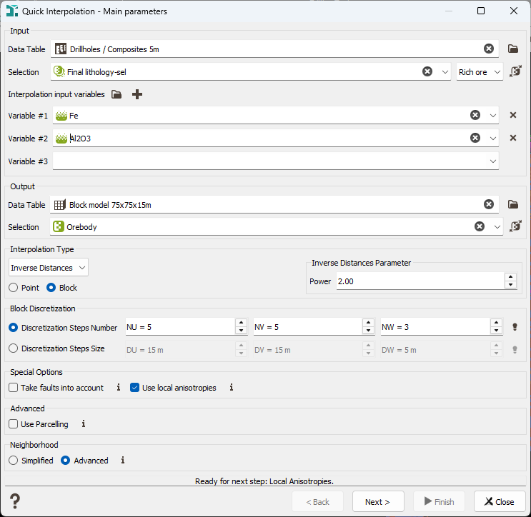
Input: The Input section corresponds to the definition of the Data Table, an optional Selection and Variable(s) used for the interpolation.
- Data Table: Click the directory icon next to Data Table to open a Data Selector and select the data table on which the Quick Interpolation task will be applied. The Data Table can also be dragged and dropped directly from the Data tab.
-
Selection: Choose an optional Selection variable to define which subset of your data you want to interpolate.
Note: The selection defines which samples can be used for interpolation, often those inside a domain. To also include samples outside the domain, you can use:
- Soft Boundaries to create a selection within a specified distance from a mesh.
- Border analysis to determine an appropriate distance using the contact analysis tool.
-
Variables: Select the variable(s) to be interpolated. There is no restriction on the number of variables as the program may interpolate as many variables as you wish, but each variable will be treated separately. Masked off samples and samples for which the values of all the specified variables are undefined are never used. The input variables must be numerical. You can also define a variable associated to an angle unit class (2D rotation) or a rotation compound (3D rotation). In this particular case of angular interpolation, only the Inverse Distances method (or the Nearest Neighbor method) will be available because it uses a dedicated algorithm.
-
Output:
- Data Table: Define here the data table where the variable(s) will be interpolated. It can be of any type but must be of the same dimension (2D/3D) as the input.
- Selection: Define here a Selection variable if you want to keep unchanged the samples outside the selection. Masked off samples are never modified.
-
Interpolation Type: Select the interpolation method to be used in the Interpolation Type list:
-
Inverse Distances: At each target point, the resulting value is calculated as the weighted average of the surrounding information (neighborhood). The weight is calculated as the inverse of a power (the Inverse Distance Power) of the distance between the data point and the target point. The weights are normalized so that the sum of all the weights equals 1.
This method is the only one which is offered (except the Nearest Neighbor method) when setting a rotation variable (i.e. a variable associated to an angle unit class or a rotation compound) on input. It performs interpolation by weight-averaging cosines and then invert the cosine to retrieve the interpolated angle. It directly uses angular data and interpolates each angle separately from the following equations:

- Nearest Neighbor: At each target point, the resulting value is equal to the value of the closest active data point contained in the neighborhood.
- Moving Average: At each target point, the resulting value is the average of the values of the active data contained in the neighborhood.
- Moving Median: At each target point, the resulting value is the median of the values of the active data contained in the neighborhood.
- Linear Kriging: This is the traditional kriging method implying the ordinary kriging method with a linear variogram. As we are only interested in the estimated value, the slope of the linear variogram model is not requested.
- Spline Kriging: This is the traditional kriging method using an Intrinsic Random Function of Order 1 (linear drift) and the (thin-plate) spline generalized covariance. As we are only interested in the estimated value, the multiplicative coefficient of the spline generalized covariance is not requested.
-
Two kinds of calculation mode are available: Point or Block. This option is only available for Inverse Distances, Linear or Spline Kriging.
- Select Point if you wish to interpolate the variable at the target point;
- Select Block if you wish to calculate interpolation of the average value of a variable over a surface/volume, called a block (generally a cell centered at the target grid node). This option may only be used if the Output Data Table is a grid.
-
- Block Discretization: In Block calculation, interpolated values are calculated over discretized points in each block. The discretization of the blocks is defined in the Block Discretization section either by entering a Discretization Steps Number or a Discretization Steps Size (regarding each direction U, V and W).
-
Special Options:
-
Take faults into account:
The faults are defined as portions of the space which can interrupt the continuity of a variable. They are introduced here to take into account geographical discontinuities in kriging interpolation (i.e. during the conditioning step). Basically, faults are used as "screens" when searching for neighbors during estimation. A sample will not be used as neighboring data if the segment joining it to the target intersects a fault.
We consider two kinds of faults:
-
2D faults which are defined as polylines (vertical faults and/or polygonal faults for faults with dip). These faults can be imported through the Vector File Import that gives you the choice of output (polygons or polylines). Polygons will be read as closed polylines in this case. With 3D data, faults will be considered as the projection of a vertical wall.
This option requires to provide the faults file (i.e. a polyline file) and an optional selection if you want to consider only a subset of your faults file. Three calculation modes are offered (only when working with 2D datasets):
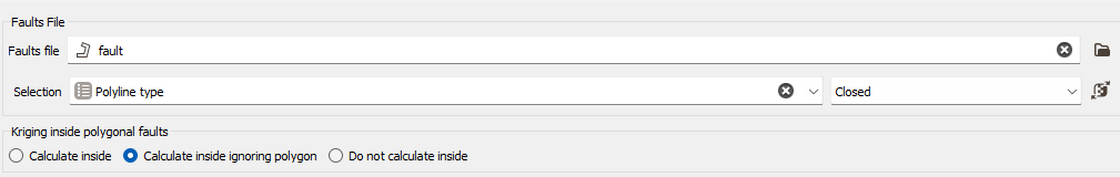
- Calculate inside: the data used in the kriging process to estimate a node inside the polygon will belong to this polygon only,
- Calculate inside ignoring Polygon: the polygonal fault will be considered as transparent for the estimation of the nodes inside the polygon,
- Do not Calculate inside: no node value will be calculated, it will be put to undefined. This allows you to consider for instance this polygonal fault as a crushed zone where no estimation is realistic or a different estimation method has to be used.
-
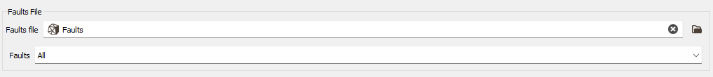
3D faults which must be defined as meshes. In this case no option is required, except the definition of the faults file and an optional selection if you want to consider only a subset of your faults file.
-
-
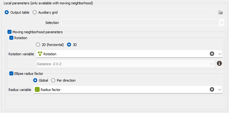
Use local anisotropies: Local GeoStatistics is an original methodology fully dedicated to the local optimization of parameters involved in variogram-based models and neighborhood ensuring a better adequacy between the geostatistical model and the data.
It is used to determine and take into account locally varying parameters to address non stationarity and local anisotropies and allows to focus on local particularities. Here, local parameters are defined for neighborhood search only. Considering local parameters will allow you to ensure that the same neighbors are used as in a kriging using local anisotropies (with same local parameters) and to see the impact of the estimation method only.
The Local Anisotropies page allows to to define local parameters for the Neighborhood.
The option requires a Grid data table on output. Variables corresponding to local parameters will be defined on the Output table or on an Auxiliary grid. They should have been previously created using Local Anisotropies functionality for example. Then you have to assign its variables to the corresponding moving parameters. You can define an optional Selection on the auxiliary grid.
Note: When choosing the Auxiliary grid mode, the local parameter will be interpolated at the target node locations. It is advised to check the output when using local rotation.
-
Select Rotation if you wish to make the neighborhood rotation varying locally.
If your input data are 3D, select 2D (horizontal) to force and define a 2D rotation. Otherwise, choose the 3D option if you wish to define a 3D rotation.
Select the Rotation variable that refers to the local rotation(s) in the local grid. To appear in the list, the variable should be associated to a Angle unit class in 2D and defined as a Rotation in 3D (see the Data Management / Create Rotation task). Be careful that the rotation is defined in the right Rotation convention.
- Select Ellipse radius factor if you wish to make the neighborhood radius varying locally. The factor can be Global, in this way the proportion between all the radius will be kept, or Per direction, to apply a factor different for each U/V(/W) direction.
Note: All the variables defined in this panel are read from the local grid. The local grid must be of the same dimension (2D/3D) as the input data file it is referring to.
-
-
-
Advanced:
-
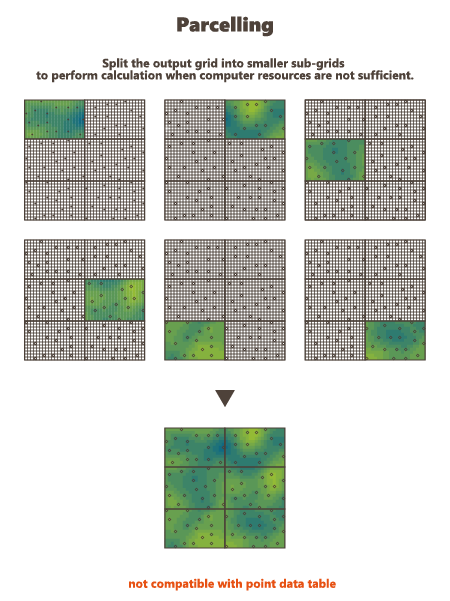
Use Parcelling:
This option is designed to split an existing grid into a given number of smaller grid files. Kriging or Simulations are performed on these sub-divisions and are finally copied on the original grid. This option is not available if the defined output data table is a points file. Using this option, you have to specify a number of split and an overlap along the axes U, V and W of the grid.
The input data are also split into new smaller point files. They will be split the same way as the grid file, but with an overlap.
-
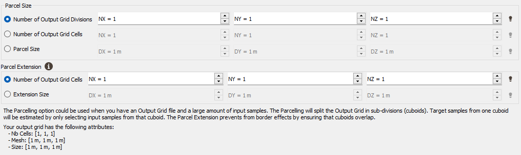
Parcel Size (U, V, W): We specify here the number of splits along the grid axes (i.e. the Number of Output Grid Divisions by default) or the size of the different sub-grids (by defining the Number of Output Grid Cells, i.e. the required number of cells of each sub-grid along each direction, or by defining the Parcel Size, i.e. the required size of each sub-grid).
Here is a 2D grid of 40 by 30 with 2 splits in U axis and 3 splits in V axis.
-
Parcel Extension (U, V, W): We specify here the overlapping in Number of Output Grid Cells or through a length with the Extension Size along the grid axes. The overlapping values apply on both side of the new grid files. This overlapping is used on the input data in order to take into account samples outside of a sub-grid but which can be involved in the neighborhood for the interpolation of a cell located on the border of the sub-grid. For this reason, we advise to consider an overlapping size at least longer than the neighborhood size. If it is not the case, an error message "The neighborhood ellipsoid size is greater than the Parcelling extension" will appear at the Neighborhood Definition step.
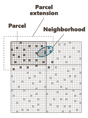
Here is the extension in dashed of a grid with an overlap of one cell along U and V.
To help you in the definition of these different parameters, a reminder of your output grid geometry (number of cells, mesh size and global extension) is displayed.
-
-
Neighborhood
In order to perform the interpolation, it is necessary to specify a search neighborhood. It indicates the rules applied for selecting the neighboring samples in the interpolation step.
Two kinds of neighborhood are available:
-
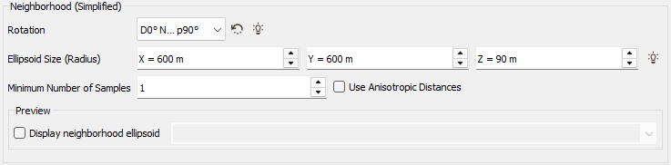
Simplified: For each non masked off sample in the output data table, the program searches for the nearest defined and non masked off sample in the input data table. If the nearest sample is contained in the Neighborhood Extension ellipse (whose the radius is defined along X/Y(Z) with an optional Rotation), the value of the input sample variable is copied into the output sample variable. The application calculates the distances between each sample and the center of gravity of the target to sort the samples. These distances can be calculated in two different ways:
- If you leave the option Use Anisotropic Distances clear (default option), the distances will be isotropic standard distances;
-
If you select the option Use Anisotropic Distances, the distances will be anisotropic and calculated taking into account the neighborhood ellipsoid parameters:

where du, dv and dw correspond to the components of the distance along the three axes of the new system, and:

where dmax is the greatest of the three distances maximum distance along u, maximum distance along v and maximum distance along w.
The anisotropic distances can be useful for example in 3D to take samples horizontally at a greater distance than vertically. All the samples located on the boundary of the ellipsoid are considered to be at the same distance from the target point, while all the samples falling outside the ellipsoid will never be selected. This principle leads distances to be distorted during the search procedure. Two points situated at the same distance from the target point will not necessary be included together in the neighborhood. As a matter of fact, all the points situated on the same ellipsoid are considered as being at the same distance from the target point.
A minimum number of neighbors can also be set in the Minimum Number of Samples box (except for the Nearest Neighbor method). If the actual number of samples that fall inside the ellipsoid is smaller than this value, the neighborhood search fails and the estimated variables at the target point receive an undefined value.
-
Advanced: a more sophisticated neighborhood can be used (like in Kriging). You may specify either a Unique neighborhood which uses all data for every output target, or a Moving neighborhood which uses a selection of the dataset.
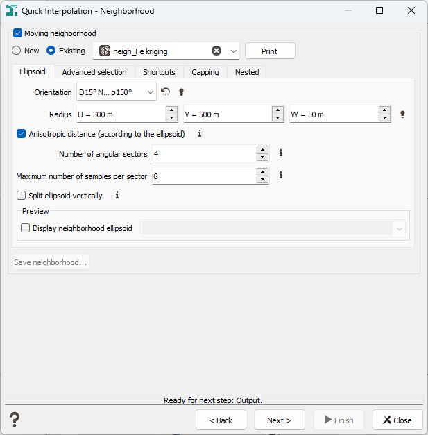
The different parameters which allow the description of a Moving Neighborhood are described in the Neighborhood Parameters Definition dialog area. Only the parameters associated to the From an Ellipsoid mode are visible. You can press the Print button to check the relevant parameters of the neighborhood (sent in the Messages window).
Output
-
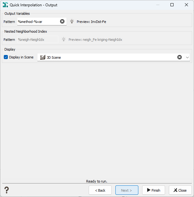
Output Variables: The objective of the Pattern parameter is to help the definition of output results names. You can edit this pattern to modify it and define the name of your choice. Click on
 to retrieve the default pattern: %method-%var
The Preview enables you to see the final name associated to the output result. If several input variables have been defined, results will be stored in as many output variables (using the defined pattern).
Note: For linear and spline kriging, a check is done before launching the calculations to automatically identify duplicate data points. The duplicate check is performed not only on the point coordinates but also on the values of the variables considered. A point is regarded as a duplicate if its coordinates are identical to another point and the variable values used for the kriging are defined.
This helps prevent matrix inversion instabilities that may lead to very bad results. In such cases, an error message will be displayed.
- Nested Neighborhood Index: This output is only available when an interpolation with a nested neighborhood is achieved (i.e. if you apply sequentially different search neighborhoods). Stores for each target point the index of the neighborhood used for the interpolation under a categorical variable (standard, nested medium, nested large, infinite, failed).
- Interpolation weights: Stores, for each target point, the sum of the interpolation weights used for the selected variable. When several input variables are defined, only the Main variable weights are saved. Click on to retrieve the default naming pattern: %var-Weights
- Display: The output interpolated variable can be displayed in a 2D/3D view in the standard way (Drag & Drop from the Data Explorer to the Map/3D view) at the end of the run. However it is possible to automatically display the result of the run by ticking the Display in Scene toggle and selecting a scene. A layer will be created in the corresponding 2D/3D scene.
-
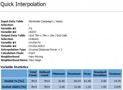
Click Finish to launch the task and interpolate all the variables. Statistics of the migrated variables are computed and displayed in the Messages window at the end of the run.