Pit Design Tutorial - Generate Contours

To prepare your project for the pit design tutorial, you need to create a series of strings that will be used to guide the automatic pit projection that takes place later on. These strings, based around one of the planning model phases, are used to constrain the eventual design.

These strings are commonly based on the contours of an isosurface within an input planning model (but they don't have to be). As they represent the zone boundaries of the optimal mining phase (say, as generated within the input model by Datamine NPV Scheduler), these are reasonable guidelines for the resulting pit excavation, at least for that particular pit/model/phase.

The contour strings used for this purpose are referred to within Studio OP and it's accompanying documentation as "constraint strings".

Prerequisites

You have completed Define Slopes.

Exercise: Generate Shell DTMs

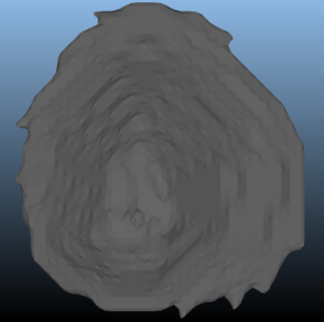
In this exercise, you will generate Shell DTM data for 2 phases in the input planning model. All of these will be generated as an isosurface of the pushback attribute information.

Using the Design ribbon, select Shell Contours.
Ensure [Design Tutorial Pit] is the selected Pit.
Ensure [P1_PH1] is the select Phase(represents "Pit 1 - Phase 1").
Make sure the default value for Subsample is 1 (data points won't be reduced).
Enter a Smooth value of 1 to smooth the result in a single pass (reducing sharp edges at cell boundaries).
Click Generate from Model to create an isosurface based on PHASE = 1:

Exercise: Generate Contours

In this exercise, you will generate a series of simple contours around the Shell DTM created above. These strings will be position according to existing bench definitions.

In the Generate Bench Contours area, ensure the Benches option is selected.
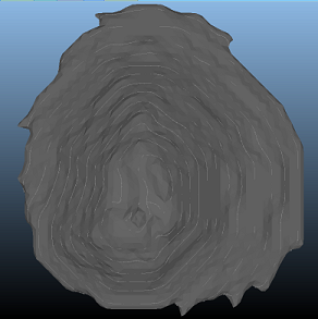
Click Generate to create and display 'raw' contours. These strings represent an exact intersection between an imaginary plane sitting on the crest of each defined bench and the shell DTM. In some cases, this is sufficient, but it can be useful to refine these strings to provide smoother and potentially more practical shapes.
Select Use splines. This allows contours to be smoothed/interpolated. Specify the following values:

Presimplify contours (remove data points before applying a spline): Set the Tolerance to "4"

Interpolated Bezier: select this option to produce curves which are formed from blended parabolas of adjacent line segments. This is the same method as used in the smooth-string command, but can result in curves which are at a significant distance from the original line segments. The default value of "4" is fine for this tutorial.

Simplify Contours (remove points within a straight line distance of another point): set the Tolerance to "0.1" (data points are sparse with the demonstration data so this value doesn't make much difference to the output.
Click Generate and note the (slight) change of string geometry resulting from splining. For a simple data set, the effect isn't that pronounced. On more complex data sets where contours can only be generated with rapid changes in vertex direction, the effect can be more obvious.
Repeat steps 1 - 4 for P1_PH23. First select [P1_PH23] from the Phase drop-down list (click Yes to save your data so far), then specify the following values for surface generation:

Phase [P1_PH2]
Subsample: 1
Smooth: 1

(Click Generate from Model at this point)

Generate Bench Contours: same values as P1_PH1: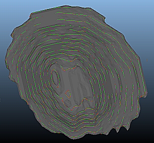
Save and Close your task. You have now created two shell DTMs, plus corresponding contour strings, for phases 1 and 23 within your planning model.

Exercise: Viewing Data with the Pit Data Control Bar

The Pit Data control bar can be used to see the status of your OP database. All managed data appears here and you can use the control bar as a menu for accessing specific data objects.

In the following exercise you are going to enable the display of the isoshell surfaces and contour strings that you generated above.

Make sure the Pit Data control bar is visible (either as a standalone control bar, or as a tab within a group). If you can't see it, check it isn't hidden using the Home ribbon's Show menu.
If the Pit Data control bar sits within a tabbed group, drag it out of the group and make it a floating dialog (this topic explains how).

If you have a secondary monitor, float the control bar onto it. The image below shows the control in its floating state, positioned to the left of the Task window - it has been resized to make it wide enough to see all Phase data table columns: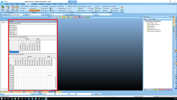
Scroll the Phase data table (the bottom one of the three) to the top so that the P1_PH1 row is visible. In the Shell DTMs and Shell Contours columns you should see unfilled circles:
These circles indicate that data exists for these project items, but are not displayed/loaded.

Left-click (once) both the Shell DTMs and Shell Contours buttons to display the relevant items in the Task window. The circles become solid and the corresponding overlay is displayed: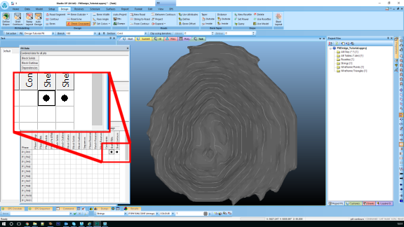
Scroll the table down so that you can see the table row for P1_PH23, then enable the same buttons:
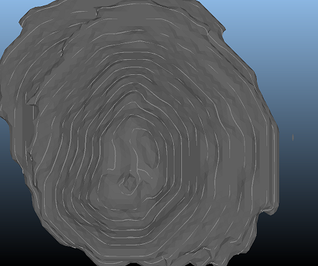
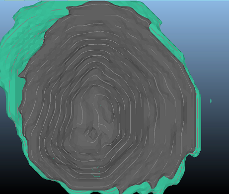
For the P1_PH23 row, double-click the Shell DTMs filled circle to reveal the Wireframe Properties dialog. This will be familiar to anyone that has used the Sheets | 3D control bar menu.
Change the Color to Fixed and select [Cyan] (or something close). Apply this to show both shell DTMs more clearly:

You can edit any 3D overlay within your OP database in this manner; double-click to access the relevant properties dialog, then apply your settings to the selected overlay.
You can also use the Pit Data bar to save generated data objects as physical files. This could be useful if you wanted to use them for other Studio operations later, such as cut and fill calculations, for example.

Right-click the P1_PH23 Shell DTM and select Save As...
Save an Extended Precision file with the default name (P1PH23SHLWIREtr.dm).
Finally, dock the Pit Data bar on the right of the screen.