Special Options
This page depends on the calculation mode and options selected on the previous page.
Block Discretization
The Block Discretization parameters are required if the Block Calculation Mode has been chosen in the previous page. This option is available in the case of block estimation on a Grid file or on a Sub-Block Model. In the second case, the Use Customized Block Sizes option will be automatically checked.
If the estimation consists in producing the optimal average value of a variable over a target block (v), the average covariance between the data point and the target cell (Cαv) as well as the average covariance of the cell (Cvv) have to be calculated. Because it is not always possible to calculate this value mathematically, the program calculates it using a discretization of the block:


where di is a discretization point and dj a randomised point.
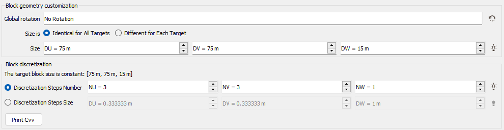
The block is regularly discretized according to the Discretization Steps Number NU, NV and NW. In this case, we define in how many cells we want to discretize the original block. The discretization can also be defined by entering the Discretization Steps Size DU, DV and DW. In this case, we define the cell size. To help you choosing the best discretization parameters, an automatic discretization is defined. This automatic value is calculated by testing different discretization steps, starting to (3,3,1) to (14,14,1). We stop to test the discretization until this one gives a covariance close to the "true" block covariance (i.e. <0.01).
To compute the average covariance of the block (Cvv), a second set of points is randomly and independently moved along X,Y and Z (50 points are selected). Of course the moving distance in a direction is smaller than the size of the block along the same direction divided by twice the number of discretizations along this direction. These moved points are only used to compute Cvv.
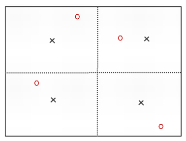
This picture shows a block discretization of two by two. Red circles correspond to random set of dj and black crosses to the centered points di.
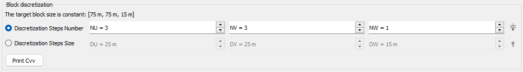
In the Kriging task, by clicking the button Print Cvv, the 10 first Cvv> results will be printed in the Messages window.
Keep in mind that a covariance or variogram is defined for data collected for a given support size and that the discretization must be coherent with the supports of both the data and the blocks. For example, if the data has been regularized on the height of the simulation bench, then the data and the block have the same extension vertically, so no discretization must be performed along Z.
Collocated Cokriging
Collocated Cokriging/Cosimulations is a particular case of cokriging/cosimulations a main variable using one or several auxiliary variables densely sampled.
The auxiliary variables are supposed to be known everywhere, i.e. at the input file sample locations and at the output file sample locations.
However the estimation at a given output file sample location makes only use of the values of the auxiliary variables collocated at this point and at the input file samples selected in the neighborhood search.
This method requires that a multivariate model be fitted to the main and auxiliary data variables, it should therefore have been specified in the Geostatistical Set.
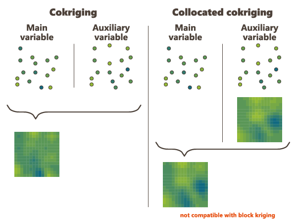
In general Collocated Cokriging is less precise than a full cokriging (making use of the auxiliary variable at all the output file sample locations when estimating each of these). Exceptions are models where the cross variogram (or covariance) between 2 variables is proportional to the variogram (or covariance) of the auxiliary variables. In this case collocated cokriging coincides with full cokriging but is also strictly equivalent to the simple method consisting in kriging the residual of the linear regression of the main variable on the auxiliary variable.
Note:If these variables are not consistent, the unbiasedness condition of Kriging no longer holds and the estimation results are unpredictable.
The Collocated Cokriging parameters are required if the Collocated Cokriging or Cosimulations Special Option has been chosen in the previous page. The objective is to inform the auxiliary variable(s) to be used for Collocated Cokriging/Cosimulations. The collocated variable(s) must match with one or several of the input data variables. It corresponds to the auxiliary variable which is defined simultaneously at the sample locations and at the target locations.
The collocated variable(s) can be located on the same output grid as the variable of interest. In this way, choose the Only Output Grid mode. Or the collocated variable(s) can be located on a different grid. In this way, choose the Only Auxiliary Grid mode and define the Data Table and an optional Selection on which the collocated variable(s) are. Then use the different selectors to indicate which collocated variable corresponds to each input variable. The variable of interest must be stay empty. If the Only Auxiliary Grid mode has been chosen, the collocated variable(s) will be interpolated on the final output grid using a bilinear interpolation.
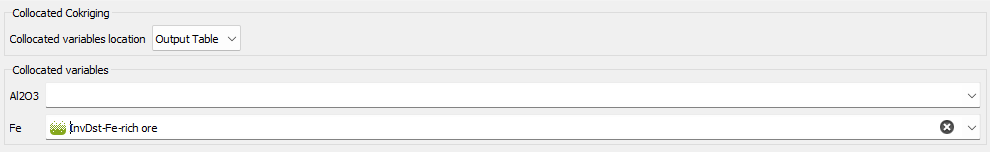
Note: Although this variable is defined in the output file, it is used as input information for Collocated Cokriging. Therefore, it must have values at target locations - no target points where the Collocated Variable is undefined will be estimated.
Rescaled Cokriging
Rescaled Ordinary Cokriging (sometimes referred as "Standardized ordinary kriging", SOCK) is a method that aims at reducing the risk of negative estimates because of negative weights assigned by Ordinary Cokriging to the secondary variables. The rescaled cokriging system replaces for n variables the n universality conditions required for unbiasedness by a single condition: the sum of all weights of all variables is equal to 1. Under the single universality condition the rescaled cokriging estimate is unbiased after having rescaled the secondary variables so that their means are equal to that of the primary variable. Consequently the values of the means of all variables must be known. Practically the means are provided exactly in the same way as for Simple Kriging (i.e. by checking the Strict stationarity option available in the Context section of the Variogram calculation in the Exploratory Data Analysis task). This option may be chosen when cokriging at least two variables.
The option is only available when a multivariate model has been fitted and strict stationarity has been specified in the input geostatistical set.
Note: This method was implemented from the following source: P. Ordinary cokriging revisited. Math. Geol. 30, 21, 1998. Goovaerts.
This method does not require any additional parameter than the means provided in the Geostatistical set.
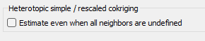
By default, if all the neighbors for one variable are undefined (heterotopic case), the estimated value is set to undefined. However, the equations can be solved even when there are no samples of the main variable and a special option is available to treat this case.
Filtering Model Components
If the model is made of several nested basic structures, you may consider that the phenomenon is a combination of several components - at different scales - which could be filtered out during the Kriging process.
By filtering out the appropriate components of the covariance part in the model, you can then estimate only the short range - high frequency - components or the long range - low frequency - components, instead of the entire phenomenon.
Moreover, this option also allows filtering out components of the drift part of the model.
Note: Filtering the Universality drift term consists in removing the contribution of the mean (either local or global depending on your Neighborhood choice). Similarly, filtering the X and Y Drift consists in removing the linear trend.
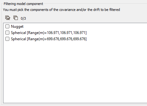
When activating the Filtering Model Components option, you have then to highlight the components of the Covariance and / or the Drift to be filtered from the model by ticking the corresponding structure(s) in the list.
Use Local Anisotropies
Local GeoStatistics is an original methodology fully dedicated to the local optimization of parameters involved in variogram-based models ensuring a better adequacy between the geostatistical model and the data.
It is used to determine and take into account locally varying parameters to address non stationarity and local anisotropies and allows to focus on local particularities.
The Local Anisotropies page allows to load the parameters required to perform Local Geostatistics (LGS).
The option requires a Grid data table on output. Variables corresponding to local parameters will be defined on the Output table or on an Auxiliary grid. They should have been previously created using Local Anisotropies functionality for example. Then you have to assign its variables to the corresponding moving parameters. You can define an optional Selection on the auxiliary grid.

Note: When choosing the Auxiliary grid mode, the local parameter will be interpolated at the target node locations. When using local rotation for neighborhoods or model, it is advised to check the output.
-
Variogram model parameters (for all structures):
-
Select Rotation if you wish to make the model rotation varying locally. This option has a sense only if the defined geostatistical set contains an anisotropic variogram model.
If your input data are 3D, select 2D (horizontal) to force and define a 2D rotation. Otherwise, choose the 3D option if you wish to define a 3D rotation.
Select the Rotation variable that refers to the local rotation(s) in the local grid. To appear in the list, the variable should be associated to a Angle unit class in 2D and defined as a Rotation in 3D (see the Data Management / Create Rotation task). Be careful that the rotation is defined in the right Rotation convention.
- Select Range factor if you wish make the different structure ranges varying locally. The ranges of the different structures will be multiplied by a given factor. This option has a sense only if the defined geostatistical set contains an anisotropic variogram model. The factor can be Global, in this way the proportion between all the ranges will be kept, or Per direction, to apply a factor different for each U/V(/W) direction.
- Select Sill factor if you wish to make the sill varying locally. The sills of the different structures will be multiplied by a given factor (in this way each structure will be modified proportionally to the global sill). This option has a sense only if the defined geostatistical set contains a multi-structure variogram model.
-
-
Moving neighborhood parameters: This section is designed to define local parameters for the Neighborhood. By default, same local parameters are defined for the variogram model and for the neighborhood. Click
 to unlock the link and to define different parameters.
-
Select Rotation if you wish to make the neighborhood rotation varying locally.
If your input data are 3D, select 2D (horizontal) to force and define a 2D rotation. Otherwise, choose the 3D option if you wish to define a 3D rotation.
Select the Rotation variable that refers to the local rotation(s) in the local grid. To appear in the list, the variable should be associated to a Angle unit class in 2D and defined as a Rotation in 3D (see the Data Management / Create Rotation task). Be careful that the rotation is defined in the right Rotation convention.
- Select Ellipse radius factor if you wish to make the neighborhood radius varying locally. The factor can be Global, in this way the proportion between all the radius will be kept, or Per direction, to apply a factor different for each U/V(/W) direction.
-
Note: All the variables defined in this panel are read from the local grid. The local grid must be of the same dimension (2D/3D) as the input data file it is referring to.
Use Uncertain Data
This option enables taking into account uncertainties associated to the input data points: either giving standard deviation measurement errors at data points in addition of the data value or providing only an interval of the data value (the exact value is unknown but we can define a lower and/or an upper bound value) (only available in the Kriging task).
-
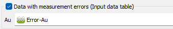
Data with measurement errors (Input data table): this option is based on a Kriging with Variance of Measurement Error (KVME). Be careful that here, in Isatis.neo, we ask for a standard deviation (with the same unit class as the input data) and not a variance.The method can be applied if one of the data variables - defined on the input file - could be considered as polluted by some particular type of noise, with the following properties:
- This noise cannot be considered as constant all over the field area - otherwise it could be modeled with a standard nugget effect in the model - Instead it is defined by its standard deviation at each sample location which will be used in the kriging system.
- It has not been taken into account while fitting a model on the data variable. The structural analysis must have been achieved on a clean subset of the polluted variable.
Choosing this option, you have to specify one or several variable that contains the amount of noise, i.e. the standard deviation, at each sample location (defined on the input Data Table).
-
Interval data: Choose this option allows you to apply a kriging with inequalities. Inequalities are defined as soft data and can be mixed with certain values defined as hard data.
Note: This option is only available when the selected geostatistical set contains a raw and a Gaussian variograms.
This methodology is actually performed in three steps:
- transformation of your hard and soft data into gaussian data.
- calculation of the conditional expectation where inequalities are defined. The method consists in running simulations running a Gibbs sampler in order to generate a set of values at each sample location with inequalities, which are consistent with the gaussian variogram model (calculated on your hard gaussian data) and with the hard and soft data. These simulated values will then be back transformed at each point to calculate their mean (conditional expectation, corresponding to the most probable values) and their standard deviation. The Gibbs sampler requires to consider all data points at the same time. Consequently, the method cannot be applied if you have more than 10 000 input samples. In this case, en error message will appear.
- kriging of your variable in a standard way using the raw hard data and the conditional expectation values at soft data locations.
In this way, this procedure has some restrictions and the Interval data option is available only if the input geostatistical set is univariate and contains an anamorphosis function and a gaussian variogram model.
- Data table: By default, the same Data table as the one of the input data is selected here. Click Use separate file to specify the input data required on another data table. Click the directory icon next to Data table to open a Data Selector and select the input data which contains the interval data. The Data table can also be dragged and dropped directly from the Data tab. You may select any type of file and activate any Selection on this file.
- Lower bound variable: select here the variable which contains, for each sample, the minimum value that the variable can take at this location. If this minimum value is Undefined, the interval has locally no lower bound or the real value is known. This variable is defined with the same unit class and the same range of values as the input raw variable. It will be then transformed in the gaussian space using the anamorphosis function stored in the geostatistical set.
- Upper bound variable: select here the variable which contains, for each sample, the maximum value that the variable can take at this location. If this maximum value is Undefined, the interval has locally no upper bound or the real value is known. It will be then transformed in the gaussian space using the anamorphosis function stored in the geostatistical set.
-
Output: The objective of the Pattern (and Context) parameters is to help the definition of output results names. You can edit this pattern to modify it and define the name of your choice. Click on
 to retrieve the default pattern: %gset-%context-withIntervalData for the Geostatistical set pattern and %var-%context-%label for the Variable pattern. "%method", "%context", "%var", "%label", "%options", "%calc", "%gset", "%groupvar", "%file" can be used for defining these patterns. The preview of the variable names enables you to see the final name associated to each output result.
Note: The algorithm could sometimes generate, during the kriging, mean and standard deviation which would give values outside of the ‘expected’ interval. It is advised to check those estimates against the input minimum / maximum values. This can be done thanks to the Conditional expectation and Stdev of measurement error variables which are saved at the end of the run.
Note: The output Geostatisical set is built in order to stored all the associated information. In this way, when selecting this Geostatistical set in the kriging task, the different options of Point kriging, Use uncertain data, Data with measurement errors and the standard deviation variable are automatically set.
-
Click Advanced parameters to access simulations parameters:
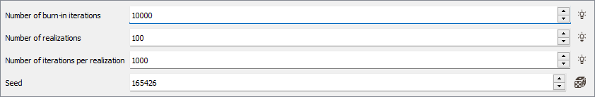
- Number of burn-in iterations: The first simulation requires a specific "burn-in" step. This step corresponds to an important number of iterations to ensure the convergence for the rest of the iterations (10 000 by default).
- In the Number of realizations box, enter the number of gaussian simulations you wish to perform by sample (100 by default). There is no theoretical limit on this number (except the performance of the machine you are working on).
- Define the Number of iterations per realization (except for the first one). The default value is set to 1000.
- The Seed corresponds to a numerical value which will be used to generate the simulations. This is an important parameter if you wish to produce twice the same simulations. There is no genuine rule for setting a seed. Nevertheless, a common practice is to define the seed as a large value (avoid 1 or 2 digit numbers). If you wish to perform a simulation producing different results, simply specify a different value for the seed. Conversely, choosing the same seed and the same number of simulations (keeping the environment unchanged) will produce identical results.
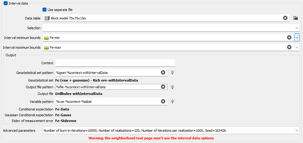
A warning is displayed to advertise you that the interval data options will not be used in the neighborhood test page
Use Customized Block Sizes
The Use Customized Block Sizes option is only available if the Block Kriging Mode has been selected and becomes compulsory if the defined output file is a points file or a sub-block file. It enables the definition of customized block sizes. The block size can be Identical for All Targets (i.e. constant) or Different for Each Target and is defined by input DU/DV/DW variables in this case. In case of a sub-block file, the block definition variable will be automatically set for each direction. A Global Rotation can also be set to the different blocks.
As the Block calculation mode is activated, the Block Discretization parameters are also required (see the Block Discretization section).
Use Sampling Density Variance
The Sampling Density Variance method is only available if the Block Kriging Mode has been selected. It provides a Mineral Resources Classification approach based on the analysis of spatial sampling density variance. This volume-like variable can be used to compare different sampling patterns in a domain or in different domains. In case of an irregular sampling pattern, it can be mapped and used to differentiate areas with different sampling densities. This method is designed to measure the quality of estimation regardless of the block size we use the Spatial density variance which is independent of the block size:

where  is the kriging variance of the volume V.
The unit of the Spatial density variance being %².m3 it makes it hard to manipulate. For that reason, the Spatial density variance is normalized by the average of the domain squared. This quantity is homogenous with a volume, it is called the Specific Volume:

This quantity is not linked to the block size nor the average value. This can help comparing estimations of different domains or deposit by solely focusing on the variogram and the sampling layout.
In order to help defining the quality of the estimation, it possible to calculate the coefficient of variation of the estimation on a given production volume:

Thresholds can be applied on this quantity to classify blocks. For instance C. Dohm defined in 2004 (“A logical approach”) thresholds of 2.5% and 5%:
- Measured: CV < 2.5%
- Indicated: 2.5% < CV < 5%
- Inferred: 5% < CV
To obtain the Spatial density variance, we need the Kriging variance  which is obtained by a Super Kriging: A super block V is defined and centered around each block v, data inside the super block is used to obtain the kriging variance of the super block
  . The Spatial density variance is then the same for the super block and the block:

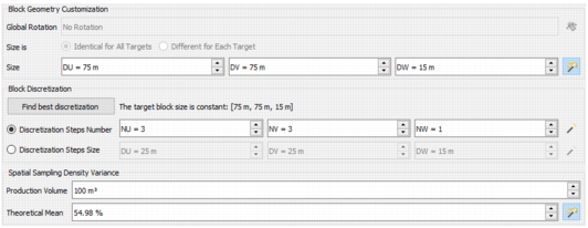
- The super blocks corresponds to production zones. Define the dimension (DU/DV/DW Size) and the Discretization (see the Block Discretization section).
- Production Volume: Specify here the production volume which will be used to calculate the coefficient of variation of the estimation.
- Theorical Mean: Specify the theorical mean which will be used to calculate the specific volume to normalize the spatial density variance.
Take Faults into account
The faults are defined as portions of the space which can interrupt the continuity of a variable. They are introduced here to take into account geographical discontinuities in kriging interpolation (i.e. during the conditioning step). Basically, faults are used as "screens" when searching for neighbors during estimation. A sample will not be used as neighboring data if the segment joining it to the target intersects a fault.
We consider two kinds of faults:
-
2D faults which are defined as polylines (vertical faults and/or polygonal faults for faults with dip). These faults can be imported through the Vector File Import that gives you the choice of output (polygons or polylines). Polygons will be read as closed polylines in this case. With 3D data, faults will be considered as the projection of a vertical wall.
This option requires to provide the faults file (i.e. a polyline file) and an optional selection if you want to consider only a subset of your faults file. Three calculation modes are offered (only when working with 2D datasets):
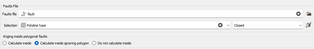
- Calculate inside: the data used in the kriging process to estimate a node inside the polygon will belong to this polygon only,
- Calculate inside ignoring Polygon: the polygonal fault will be considered as transparent for the estimation of the nodes inside the polygon,
- Do not Calculate inside: no node value will be calculated, it will be put to undefined. This allows you to consider for instance this polygonal fault as a crushed zone where no estimation is realistic or a different estimation method has to be used.
-
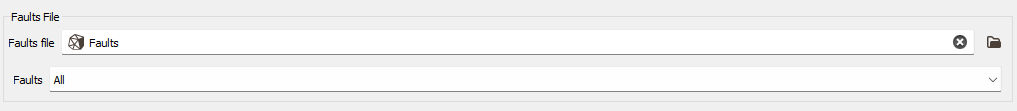
3D faults which must be defined as meshes. In this case no option is required, except the definition of the faults file and an optional selection if you want to consider only a subset of your faults file.
Multiple kriging
This method enables you to krige all the components / indicators at once when selecting a geostatistical set made from a macro variable built through PCA/MAF, PPMT or MIK Pre-processing. It is not compatible with all the other options and transformations (gaussian or residual variable).
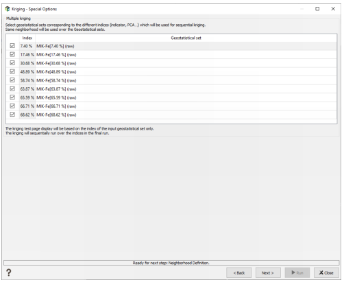
The special option page lists all the component / indicator values and the corresponding geostatistical sets that will be used for the kriging. If the input geostatistical set is built from the MIK Pre-processing task, the matching between the different indicators and the geostatistical sets will be made automatically. For the PCA/MAF and PPMT components, you will have to select the different geostatistical sets manually. Select the indices you want to krige.
The same neighborhood is used to krige all the components / indicators. Note that the capping is not available. The neighborhood test is applied on the input geostatistical set only.
The Run loops over the different geostatistical sets, and creates one macro variable in the output data table, with one kriged component / indicator per index. The statistics of the kriged components / indicators are printed in the Messages window.
Reset negative weights to zero
The aim of this option consists in resetting negative weights values to zero in Ordinary Kriging and Simple Kriging. Modifying the weights generally avoids getting values outside the original range of values (greater than the minimum input value and smaller than the maximum input value).
Negative weights are set to zero. If the sum of weights is greater than one, then the weights are rescaled so that they sum to one. In the Ordinary Kriging case, this will always lead to rescaling (because the sum of weights started at one, and the elimination of negative weights makes the sum greater than one). In the Simple Kriging case, this may or may not lead to a rescaling.
The result of this option on the kriging weights can be visualized in the neighborhood test page. Check the Print Test Target Information in Messages toggle to print all the information related to the tested target, and particularly the weight of each sample considered in the neighborhood.
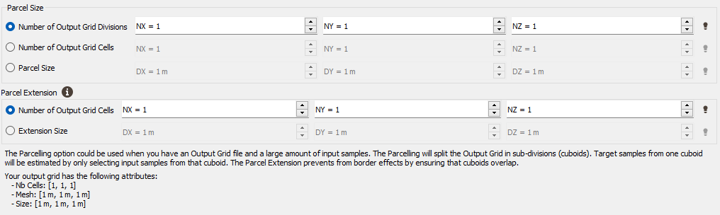
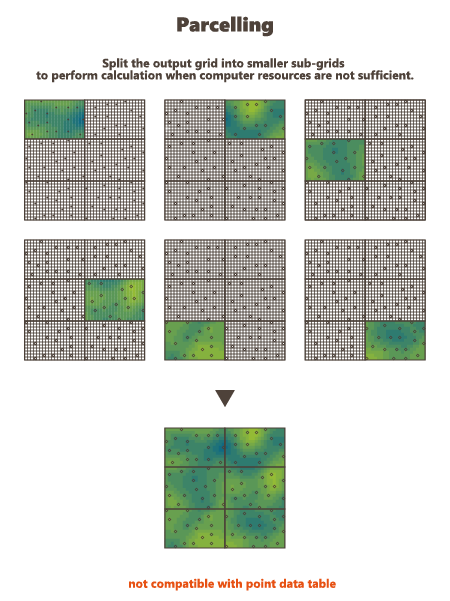
Use Parcelling
This option is designed to split an existing grid into a given number of smaller grid files. Kriging or Simulations are performed on these sub-divisions and are finally copied on the original grid. This option is not available if the defined output data table is a points file. Using this option, you have to specify a number of split and an overlap along the axes U, V and W of the grid.
The input data are also split into new smaller point files. They will be split the same way as the grid file, but with an overlap.
-
Parcel Size (U, V, W): We specify here the number of splits along the grid axes (i.e. the Number of Output Grid Divisions by default) or the size of the different sub-grids (by defining the Number of Output Grid Cells, i.e. the required number of cells of each sub-grid along each direction, or by defining the Parcel Size, i.e. the required size of each sub-grid).
Here is a 2D grid of 40 by 30 with 2 splits in U axis and 3 splits in V axis.
-
Parcel Extension (U, V, W): We specify here the overlapping in Number of Output Grid Cells or through a length with the Extension Size along the grid axes. The overlapping values apply on both side of the new grid files. This overlapping is used on the input data in order to take into account samples outside of a sub-grid but which can be involved in the neighborhood for the interpolation of a cell located on the border of the sub-grid. For this reason, we advise to consider an overlapping size at least longer than the neighborhood size. If it is not the case, an error message "The neighborhood ellipsoid size is greater than the Parcelling extension" will appear at the Neighborhood Definition step.
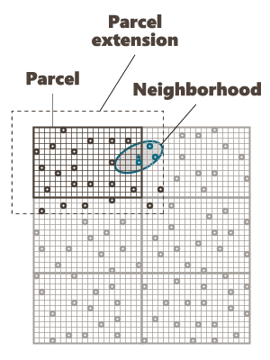
Here is the extension in dashed of a grid with an overlap of one cell along U and V.
To help you in the definition of these different parameters, a reminder of your output grid geometry (number of cells, mesh size and global extension) is displayed.