MIK Pre-processing

The goal of this tool is to create a macro variable containing indicators, at selected indicator values (thresholds), of an input variable. An indicator is equal to 1 if the input variable is greater than or equal to a threshold, and zero if the input variable is less than a threshold.

The main interface is divided into two areas: on the left are the parameters and on the right are the graphics and statistics table to help the user choosing suitable indicators and parameters.

Input

Data Table: The data table that contains the input variable and will contain the indicators.
Selection (optional): Restrict the calculation to a selection.
Weight (optional): Apply a weight to the raw variable.
Raw variable: The input variable from which the indicators will be calculated.

Indicator Definition

Number of indicators: Select the number of indicators to be automatically calculated. This field is only accessible when using the automatic values for indicators or quantiles. The default number is 10.
There are two ways of choosing the indicator values:
- Indicator values: set the values of the indicators by editing them or using the automatic values (the quantiles below are updated accordingly). The algorithm to compute the automatic indicator values starts with indicators at percentiles 1-99, and then repeatedly removes the indicator which causes the smallest summed absolute error of a linear approximation to the full CDF.
- Quantiles: set the values of the quantiles by editing them or using the automatic values. The corresponding indicators will be calculated accordingly.
  
  Click on to set default values for the lists.
  
  Click Edit to pop up the Value Definition window and customize the list of indicators and quantiles.
Local histogram interpolation parameters:

The number of indicators only give a relatively small number of points in the cumulative distribution function. To calculate statistics, the full distribution is needed, and that requires interpolating between indicators, and extrapolating the tails. The parameter choices made here can have a substantial impact on the results, in particular for upper tail when the original data is highly right-skew.

The impact of the parameters is visible on the cumulative histogram on the right hand side of the interface. The aim is to make the interpolated distribution (in red) matching the raw one (in blue).

The statistics printout from MIK Pre-processing in the Messages window gives some possible values for the exponents, but does not say if one model or another is a better fit to the data.

Note: These transformations of the indicator Kriging results have been inspired by the GSLIB methods and we strongly recommend the user to refer to the paragraph V.1.6 "Going Beyond a Discrete CDF" of the GSLIB User Guide (Deutsch and Journel - Oxford 1992) to understand the methodology and the corresponding parameters.

There are four types of interpolation models offered. In the following descriptions, z₁, z₂,…, z_n are the indicator thresholds, and F(z) is the cumulative distribution function, i.e., the probability to be less than or equal to z. The Kriged indicator for z_i is 1-F(z_i), and the formulas below describe the interpolation between consecutive thresholds z_i and z_i+1.
- Linear Model:
  
  This is a linear (straight line) interpolation between points on the cdf, corresponding to a uniform distribution between z_i and z_i+1.
- Power Model:
  
  The exponent α must be greater than zero.
  - α < 1: Right-skew distribution between z_i and z_i+1.
  - α = 1: Uniform distribution; identical to linear model interpolation.
  - α > 1: Left-skew distribution.
- Beta Power Model:
  
  The exponent β must be greater than zero. This model is effectively a mirror-reversed version of the power model. When β>2, the modelled histogram will smoothly decay to zero at the upper bound of the interval.
  - β < 1: Left-skew distribution between z_i and z_i+1.
  - β = 1: Uniform distribution; identical to linear model interpolation.
  - β > 1: Right-skew distribution between z_i and z_i+1.
- Hyperbolic Model:
  
  This model is only used for the extrapolation above the last indicator z_n (which must be positive), i.e., for the upper tail. Outside of geostatistics, it is usually known as the Pareto distribution.
  
  Unlike the linear and power models, this distribution is unbounded, with the cdf only asymptoting to 1, never actually reaching that value. The exponent α controls how fast cdf approaches 1, or equivalently how long the tail is - a smaller value of α gives a longer tail and a higher mean (e-type estimate). The exponent must be greater than 1.
  - 1 < ɑ ≤ 2: The mean of the distribution is finite, but the variance is theoretically infinite. (An output standard deviation variable will nevertheless be finite, because of the finite number of discretization steps used in the calculation.)
  - α > 2: Both the mean and variance are finite.
The extrapolation concerns the lower tail, the upper tail, and also between the indicators (within-classes).
- For the Lower tail extrapolation, a power model exponent is chosen so that the power model's expectation is equal to the mean of the input variable below the first indicator value, assuming that the minimum allowed value in the power model is the minimum of the input variable. If the bounds of the power model are [z_min,z_max], and the data mean within this interval is m, then the exponent α is set by:
  
  The lower tail extrapolation uses a power model with an exponent of 1 by default.
- For the Within-classes extrapolation, a linear model is used by default.
- For the Upper tail extrapolation, there are three exponents listed.
  - A power model exponent, set so that the power model's expectation is equal to the mean of the input variable at or above the final indicator value, assuming that the maximum allowed value in the power model is the maximum of the input variable. The details of this calculation are the same as for the power model in the lower tail.
  - A hyperbolic model exponent, set so that the expectation of the hyperbolic model is the mean m of the input data at or above the final indicator value z_n_n:
  - The maximum-likelihood estimate of the hyperbolic model exponent, calculated from all input variable values z_i greater than or equal to the final indicator value:
  The upper tail extrapolation uses a hyperbolic model with an exponent of 5 by default.
Different interpolation choices can be made for three cases:
- Lower Tail: Choice of linear model, power model, and beta power model; extrapolation will be between the Minimum Value Allowed and the first indicator threshold. A power model is a common choice. The Minimum Value Allowed defaults to the first indicator threshold, and would usually be replaced by the minimum of the original variable.
- Within-Classes: Choice of linear model, power model and beta power model; this is the interpolation between indicator thresholds. The linear model is a common choice.
- Upper Tail: Choice of linear, power, beta power and hyperbolic models. In the case of the linear, power and beta power models, extrapolation is between the last indicator threshold and the Maximum Value Allowed, at which point the cdf reaches 1. For the hyperbolic model, which is unbounded, this maximum is ignored. The choice of model and exponent here is often the most critically important. Guessing exponents without studying the distribution of your original variable may lead to drastic over-estimation of the mean grades or metal quantity above a cutoff.
A hyperbolic model is common when the original variable is highly right-skew, i.e., there is a long tail of high values, as is often the case in gold.

A stylised graphical example of such interpolation is shown below, using only four indicators. A power model (exponent 3) is used between zero and the first indicator, a linear model is used between indicators, and a hyperbolic model (exponent 4) is used above the last indicator.

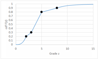
Note: You will see that the interpolation parameters chosen on the left are interactively applied to the interpolated distribution on the right. In the graphic, the raw distribution is printed in blue and the interpolated one is displayed in red, with the diamonds corresponding to the indicator values. The aim is to make the two curves matching.

Graphics and statistics

On the right hand side of the interface are printed graphics and statistics to help the user making the best choices.

Cumulative histogram

The cumulative histogram displays the raw distribution in blue, and the interpolated distribution in red. The red diamonds correspond to the defined indicator values. The user should make the two curves matching.

The local histogram interpolation parameters defined on the left will impact the interpolated curve between the indicators:
- lower tail corresponds to the line from the beginning of the distribution to the first indicator;
- within-classes corresponds to the line between two indicators;
- upper tail corresponds to the line from the last indicator to the end of the distribution.
Remember that flying your mouse on a graphic window makes appear a tool bar where actions may be selected (for more information, see the documentation on Graphical Options).
Statistics table

The table prints the statistics of the different defined classes. Each class is defined from two indicator values (but the first and last classes which go to -/+inf.). The columns are:

Class: the lower and upper bounds of the class
Count: the number of samples within the class
Quantile: the quantile value for the upper bound of the class
Metal percentile:

Let w_i and z_i be the weights and grades of the samples. Define Q0 = sum(all samples) w_i * z_i. Then the metal percentile corresponding to a grade value zc is:

Q_percentile = [sum(samples with grade <= zc) w_i * z_i] / Q0
Mean: the mean value of the samples within the class
Median: the median value of the samples within the class
Mean (interpolation): the mean value between the lower and the upper bound of the class
Error: the percentage of difference between the mean and the interpolated mean.

The graphics and tables can be saved in a Chart File using this particular format (using the Store Chart File button available in the task window).

Output

Macro Variable: Enter the name for the macro variable that will store the indicators. Also, it can be defined using a pattern. The default pattern is MIK-%var. A preview below shows the final name of the indicator variable.

If the output macro variable already exists, it will be deleted before the run if existing indicators are different from the defined indicators. If an existing output has been selected but the defined indicators are different, a warning window will pop-up to advise the user.
Display: Activate the option to display the first indicator of the output macro variable in the selected scene.

Run

The main output is the macro variable of the indicators. This variable will be stored in the data table defined in input (same location as the raw variable). In addition to the statistics of these indicators, there are also some suggested choices of exponent for the lower tail and upper tail extrapolation which are printed in the Messages window.