Interface

• Interface
• • Main Parameters
  • 2D Constraint and Local Parameters
  • • Local Parameters
    • 2D Constraint Parameters
  • Algorithm and Output Parameters

Main Parameters

• Input Data:

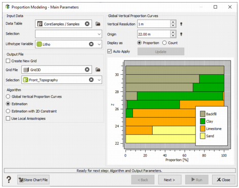
  • Data Table: Click Data Table to open a Data Selector to select the data where the lithotype information has been stored. The Data Table can also be dragged and dropped directly from the Data tab. It can be 2D or 3D and of any geometry (points, boreholes assays...).
  • Selection: Optional choice of the selection (as a restriction of the input Data Table) to apply the Proportions Modeling task.
  • Lithotype Variable: Select the categorical variable corresponding to the lithotype from which proportions will be computed. As mentioned in the introduction, the output of the task is a macro-variable, indexed from the lithotype variable catalog, containing the local proportions of each category of the lithotype.

• Output File:

  • Create New Grid: If not activated, the output proportion results will be stored on an existing grid of the same dimension as the input file.

    Click Grid File to open a Data Selector to select the your output grid. An optional Selection can be defined on the grid to restrict the estimation. If the Create New Grid option is activated, the output grid is generated on-the-fly to cover the input data. In this case, it is possible to defined the Grid Geometry by setting a Mesh size (along U, V and W) and a Rotation.

    The Origin and the Number of Cells are indicated for information. In order to visually check the grid adjustment with input data (and optionally the simulation grid), a Preview in a scene of the Map/3D Viewer is proposed.

• Algorithm: the task offers three algorithms.

  • Global Vertical Proportion Curves: The Vertical Proportion Curves (VPC) are used to interpret the vertical variability of the lithotypes (facies or lithofacies) in a deposit. This tool is very useful for the geologist as it gives an idea of the original (before deformation) distribution of the facies. The lithostratigraphy can be studied to understand the deposit genesis.

    This method consists in directly computing the proportions, for each layer of the output grid. Hence, it assumes that the proportions are horizontally invariant. A smoothing algorithm can be used in order to vertically spread the raw proportions.

  • Estimation: This method consists in performing an estimation from log-likelihood. The log-likelihood cost function contains at least two terms: the former corresponds to the contribution of data (transformed into gaussian threshold, the latter corresponds to the contribution of a Matern 2 structure which is introduced in order to add some spatial structure / continuity in the estimation. It is based on binary optimization, using gaussian threshold. Hence, the idea is to build a tree of lithotypes group and complementaries, and to perform binary optimization to estimate the proportions of each group versus its complementary. To illustrate this idea, let us consider 4 lithotypes: A, B, C and D. The main calculator will perform the following sequence:

    • A vs [B C D] --> pA / (1-pBCD) (in whole lithotypes)
    • B vs [C D] --> pB / (1-pCD) (in BCD group)
    • C vs D --> pC / (1-pD) (in CD group)

    Then, as it is composed variables, the idea is to perform the adequate multiplications to retrieve the global value of pD from pCD and pBCD. This method is based on SPDE and thus is compatible with local geostatistics (LGS).

  • Estimation with 2D Constraint: This is the same method as above, but introducing a new term corresponding to the seismic data into the log-likelihood cost function. The method consists in adjusting the already calculated proportions according to the average proportion of a subset of lithotypes constrained over the whole unit height.
  • Use Local Anisotropies: This option is enabled only if using the Estimation algorithm has been chosen.

• Global VPC: The Vertical Proportion Curves (VPC) are used to interpret the vertical variability of the lithotypes (facies or lithofacies) in a deposit. This tool is very useful for the geologist as it gives an idea of the original (before deformation) distribution of the facies. The lithostratigraphy can be studied to understand the deposit genesis. The VPC is a very simple tool which calculates, for each level of the working grid, the number of occurrence of each facies. This VPC can be normalized to get a proportion for each lithotype.

  • Vertical Resolution: Enter here the resolution required for your vertical proportions. The default value is a ratio of the input data bounding box if no simulation grid is provided and is equal to the Z cell size if provided.
  • Origin: Specify the grid origin of you want to align your vertical proportions with a particular Z level.

  • Display as: If the input dataset is 3D, the non-smoothed Global VPC is displayed. It simply consists in computing the global proportions of the different lithotype categories for each layer of a 3D grid covering the input data. The proportions are assumed horizontally invariant. Hence, the proposed graph is a 2D graph, whose Y-axis represents the Z-coordinates of the grid cells (layer elevation) and abscissa represents the proportions of the different lithotypes in this layer. The Global VPC can be parametrized with:

    • Proportion: Simply display of the computed proportions, whose sum is equal to 1.
    • Count: Display of the number of lithotype occurrences in each layer. This option can be interesting in order to detect layers where few data are available.
  • Check the Auto Apply option to automatically apply modifications of one of the above-described parameters or click on the Update button each time you want to apply the modifications on the VPC graph.

Remember that flying your mouse on a graphic window makes appear a tool bar where actions may be selected (for more information, see the documentation on Graphical Options).

The graphic can be saved in a Chart File using this particular format (using the Store Chart File button available in the task window).

2D Constraint and Local Parameters

This optional page is proposed if the Estimation with 2D Constraint method is used or if the Use Local Anisotropies option is checked. If any of these two options is not used, we will automatically go the last Algorithm and Output Parameters step.

Local Parameters

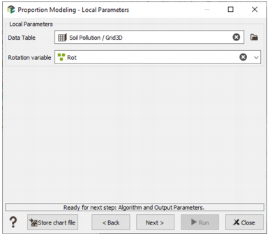
Local GeoStatistics is an original methodology fully dedicated to the local optimization of parameters involved in variogram-based models ensuring a better adequacy between the geostatistical model and the data. It is used to determine and take into account locally varying parameters to address non stationarity and local anisotropies and allows to focus on local particularities.

Here, as the structure is supposed homogeneous in terms of sills and ranges in the whole field, only the rotation is required. The local rotation parameter can be calculated thanks to the Local Anisotropies functionality.

• Data Table: Define the Data File associated to the grid containing the local structure rotation.
• Rotation variable: Select the Rotation variable that refers to the local rotation(s) in the local grid. To appear in the list, the variable should be associated to a Angle unit class in 2D and defined as a Rotation compound in 3D (see the Data Management / Create Rotation task). Be careful that the rotation is defined in the right Rotation convention.

Note: When choosing a local grid file different from the grid defined to store the output proportions, the local rotation will be interpolated at the target node locations. It is advised to check the output.

2D Constraint Parameters

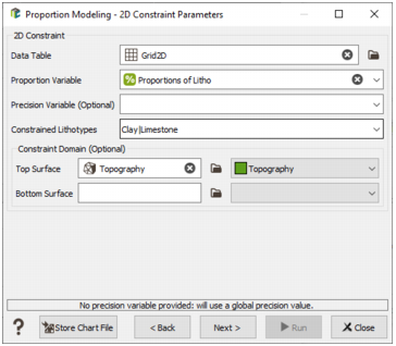
This page enables the setting of the 2D Constraint to add an external information on a subset of lithotypes proportions on a whole pillar. For example, if it is defined for a group of lithotypes AB in the previous ABCD example, the constraint means that mean_z(pA + pB)[ix, iy] = constraint[ix,iy] for ix=1,...,nx and iy = 1,...,ny.

• Data Table: Click Data Table to open a Data Selector to select the 2D constraints grid file where the proportions have been stored. The Data Table can also be dragged and dropped directly from the Data tab.
• Proportion Variable: Select the proportion variable corresponding to the constraint local evaluation for each data table cell and used to adjust the VPC modeling. As it is a proportion, this variable has to be bounded by 0 and 1.
• Precision Variable (Optional): This variable is optional. It enables the setting of the confidence level on each local value. Providing a precision value is important for the log-likelihood estimation. If no local value is known, a global one can be provided in the last page.
• Constrained Lithotypes: Select in the list the input lithotypes on which applying the constraints.
• Constrained Domain (Optional): Optional surface mesh enables the definition of a domain in which applying the constraint. You can provide either just a Top Surface, or just a Bottom Surface surface or both surfaces.

Note: If the 2D constraint is used, the estimation algorithm firstly estimates the constrained lithotypes group proportions versus the others, and then apply the standard splitting strategy on the constrained lithotypes and finally unconstrained lithotypes in order to compute individual proportions.

Algorithm and Output Parameters

• Use Smoothing for Global VPC: This option is only available if you have chosen the Global VPC algorithm. If activated, it enables to vertically spread the raw proportions. The smoothing consists in averaging a proportion value at for the IZ layer with the (IZ - 1) and (IZ + 1) values.

  • Number of Iterations: It corresponds to the number of iterations of the smoothing algorithm. The higher the number of iterations, the smoother but the less accurate (regarding input data) the output proportions.

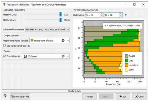
• Estimation Parameters: These parameters are only available if you have chosen the Estimation (with 2D Constraint) algorithm.

  • The two following sliders enable to set the weight / confidence level on:

    • Model vs Data: The higher this precision (closer to 1), the smoother and the more spatially continuous the output proportions.
    • 2D Constraint: The higher this precision, the higher the impact of 2D Constraint (when using a variable in the 2D Constraint file in order to define local precision values).

  • Advanced Parameters: Click on the list to access several advanced estimation algorithm parameters.

    • Model Ranges: It corresponds to the ranges along U, V and W directions used for the Matern 2 structure (used in order to generate the SPDE kriging interpolator).
    • Use Local Parameters: This option is only available if the Use Local Anisotropies option has been checked before. It allows to quickly activate/desactivate the option without going back to the previous page.
    • Use 2D Constraint: This option is only available if the Estimation with 2D Constraint algorithm has been chosen before. It allows to quickly activate/desactivate the 2D constraint without going back to the previous page.

    • Convergence Parameters: The estimation method is based on a two-level iterative numerical algorithm: Maximum Likelihood Optimizer and Conjugate Gradient. The convergence parameters can be modified:

      Precision: Negative integer corresponding to the exponent for the algorithm tolerance. For example, a precision = -2 leads to a 1.e-2 tolerance.

      Max Number of Iterations: Maximum number of iterations of the algorithm to perform. The default values are respectively set to 10 and 100 for the Maximum Likelihood Optimizer and for the Conjugate Gradient.

• Output Variable:

  • Proportions Macro Variable: Enter here the name of the variable which will contain the output proportions. By default, the created variable will be named Proportions of LithotypeVariableName. Proportions will be stored in a macro variable with one index per lithotype.
  • Store into Constraint File: This option is only available if the Estimation with 2D Constraint algorithm has been chosen before. It enables to store the evaluation of the constraint from estimated proportions into the constraint file (for validation purposes for instance).
• Select the Display toggle to display the output proportion of the first lithotype (first index of the macro variable) calculated in the output grid in a defined scene (2D or 3D) at the end of the run.
• Vertical Proportion Curves: The output Vertical Proportion Curves using the output proportions are displayed only in 3D. If an output selection or the Estimation algorithm has been used, you can select the grid indices (IX,IY) of the 3D grid pillar to display.