Main Parameters

• Main Parameters
• • Input Geostatistical Set
  • Input File
  • Output File
  • Calculation Mode
  • Special Options
  • Neighborhood
  • Advanced

Input Geostatistical Set

Select here your Input Geostatistical Set which contains geostatistical parameters required for kriging: variogram model, anamorphosis (to apply the back transformation from the gaussian variable(s) to the raw variable(s)), stationarity option (to apply ordinary kriging, simple kriging, or to use drift(s)) and input variable(s) you want to interpolate. A Print button enables you to check the content of the Geostatistical Set defined (sent in the Messages window).

Note: A check is done on multivariate geostatistical sets to protect from numerical instabilities while kriging. This kind of problem can happen when the cross-variogram model is very close to perfect correlation between the variables. In this case, a warning message is printed in the status bar at the bottom of the interface. The same check and an automatic correction is offered in the fitting of the Exploratory Data Analysis.

Input File

In the Input File you can see displayed information depending on your input geostatistical set: Data Table, an optional Selection which you may modify, Variable(s) used for the kriging and Stationarity Option. Depending on the content of your geostatistical set, you will have different options to store the output variable(s), transformed or not:

• Estimate Raw Variables: Choosing this option allows you to perform the estimation of the raw variable(s).

  • Standard case: Your Geostatistical Set contains the raw variogram, and this variogram will be used to perform the kriging.
  • Drift case: Your Geostatistical Set contains the variogram for residuals which will be used to perform non-stationary kriging (UK) or kriging with a known drift.
  • Gaussian case: Your Geostatistical Set only contains a gaussian variogram model which will be used to perform the kriging and the back transformation will be applied. This option is only compatible with Point Kriging.
• Estimate Gaussian Variables: This option is only available when a gaussian anamorphosis and a gaussian variogram model have been specified in the Input Geostatistical Set. Choosing this option allows you to directly store the gaussian estimation in output (the back transformation is not applied to calculate the raw estimate(s)).
• Estimate Residuals: This option is only available when a drift has been specified in the Input Geostatistical Set. Choosing this option allows you to directly store the residuals estimation in output (the drift is not added to calculate the raw estimate(s)).

• Estimate Conditional Expectation: This option, also known as multigaussian kriging, is only available when a gaussian anamorphosis and a gaussian variogram model have been specified in the Input Geostatistical Set. Choosing this option allows you to calculate the estimation through a conditional expectation (instead of a kriging) and to access additional results such as quantiles, confidence intervals, probability of exceeding a threshold, etc.

  A block anamorphosis is required to access the Block Kriging mode. This one is calculated using the DGM2 method available in the Support Correction tool.

  Conditional expectation is only compatible with local parameters and faults options. It is not compatible with the Capping option in the Neighborhood Definition (the tab is visible but greyed out, the option will not be used even if it is checked).

  When applying simple kriging in multivariate, a special option is available to treat the heterotopic case (the same as for the rescaled cokriging).

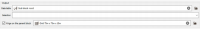
Output File

Select the Output Data Table on which you want to store the kriged estimate(s). It can be of any type (points, boreholes, grid, sub-blocks). You may define a Selection on the output samples - useful when the data is heterogeneous and when several steps should be processed one after the other, using different models and/or neighborhoods.

Particular case of the sub-blocks:

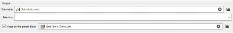
• Krige on the parent block: In the case where the output data table is a sub-block model, you have the option to perform the kriging on a regular (coarser) grid file named "the parent blocks". (To justify the existence of this option, kriging the sub-block model is not a recommended geostatistical practice.)

  

  • Definition of the parent grid (i.e. a regular grid):

    • If you already have the parent grid, you can select it with the data selector. The dimension (2D or 3D) and the location must match the sub-block model characteristics.

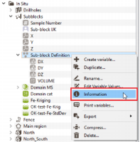
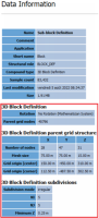
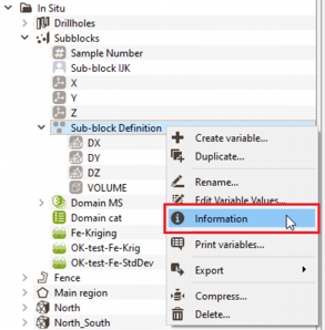
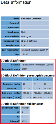
    • If you do not have the parent grid, but the sub-block definition contains the parent grid geometry, then you can leave the field empty, and a temporary parent grid will be created. To check if the sub-block definition contains this information, right-click on it and choose Information.

      

Note: If the sub-block model does not follow a regular grid (sub-blocks after an unfolding for example) or if the parent grid geometry is not defined in the sub-block definition, providing a parent grid is mandatory to krige on the parent blocks.

The neighborhood test (done in the Neighborhood definition page) is done using the parent grid. The kriging will then be performed on the parent blocks and the results are copied onto the sub-blocks (using internally the Copy Using ID tool). The output variables are saved in the sub-block model only.

Calculation Mode

Kriging can provide different types of results depending on the selected option:

• Select Point Kriging if you wish to calculate kriging of the variable at the target point;

• Select Block Kriging if you wish to calculate kriging of the average value of a variable over a surface/volume, called a block (generally a cell centered at the target grid node). This method is not compatible with the definition of drift(s) (associated to the Input Geostatistical Set).

  In Block Kriging, average variogram values are calculated over discretized points in each block. The discretization of the blocks is defined in the Special Options either by entering a Discretization Steps Number or a Discretization Steps Size (regarding each direction U, V and W).

Special Options

You may activate special options in order to perform particular types of kriging:

• Collocated Cokriging: This method is only available when a multivariate model has been fitted and has been specified in the Input Geostatistical Set. It is a particular case of cokriging, using one or several auxiliary variables densely sampled. The auxiliary variables are supposed to be known everywhere, i.e. at the input file sample locations and at the output file sample locations. It requires the definition of collocated variables on an auxiliary grid file, in this case values of collocated variables will be estimated on the output grid by a bilinear interpolation, or directly on the output grid. These variables must match the variable(s) that are specified in the input data table.
• Rescaled Cokriging: This method is only available when a multivariate model with a strict stationarity has been fitted and has been specified in the Input Geostatistical Set. It aims at reducing the risk of negative estimates because of negative weights assigned by Ordinary Cokriging to the secondary variables.
• Use Local Anisotropies: This method enables to take into account locally varying parameters (model rotation, sill, range of the variogram model and/or rotation, radius of the neighborhood) to address non-stationarity and local anisotropies ensuring a better adequacy between the geostatistical model and the data. The method is not compatible with the use of a unique neighborhood. It requires a Grid data table on output. Variables corresponding to local parameters will be defined on the output grid or on an auxiliary grid.
• Use Customized Block Sizes: This option is only available if the Block Kriging Mode has been selected and becomes compulsory if the defined output file is a points file. It enables the definition of customized block sizes for a points file. The block size can be constant or different for each target and is defined by input DU/DV/DW variables in this case.
• Filtering Model Components: If the model is made of several nested basic structures, you may consider that the phenomenon is a combination of several components, at different scales - which could be filtered out during the estimation process. It is also possible to filter drift(s) contained in the Input Geostatistical Set. It requires defining the structure(s) of the variogram and/or the drift(s) to be filtered.
• Use Uncertain Data: This option enables taking into account uncertainties associated to the input data points: either giving standard deviation measurement errors at data points in addition of the data value or providing only an interval of the data value (the exact value is unknown but we can define a lower and/or an upper bound value).
• Use Sampling Density Variance (Super Kriging): This method is only available if the Block Kriging Mode has been selected. It provides a Mineral Resources Classification approach based on the analysis of spatial sampling density variance. This volume-like variable can be used to compare different sampling patterns in a domain or in different domains. In case of an irregular sampling pattern, it can be mapped and used to differentiate areas with different sampling densities.
• Take Faults into account: This method enables taking into account geographical discontinuities in kriging interpolation. Basically, Faults are used as "screens" when searching for neighbors during estimation.
• Multiple kriging: This method enables you to krige all the components / indicators at once when selecting a geostatistical set made from a macro variable built through PCA/MAF, PPMT or MIK Pre-processing. It is not compatible with all the other options and transformations (gaussian or residual variable).
• Reset negative weights to zero: The aim of this option consists in resetting negative weights values to zero in Ordinary Kriging and Simple Kriging. Modifying the weights generally avoids getting values outside the original range of values.

Neighborhood

In order to perform the kriging, it is necessary to specify a search neighborhood. It indicates the rules applied for selecting the neighboring samples in the kriging step.

You may specify either a Unique Neighborhood which uses all data for every output target, a New Moving neighborhood or an Existing Moving which uses a selection of the dataset. Parameters of this neighborhood has been defined in the Neighborhood Definition step.

You can press the Print button to check the relevant parameters of the neighborhood (sent in the Messages window).

Advanced

• Use Parcelling: This option enables you to deal with a large amount of input samples or for per-layer estimation. The parcelling will split the grid into smaller sub-grids of a given size. The input data table will be split in the same way including overlapping areas. Kriging is performed on these sub-divisions and are finally copied on the original grid. This option is not available if the defined output data table is a points file.