Uniform Conditioning (UC)

UC Overview

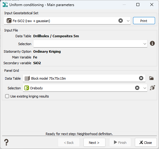
The Uniform Conditioning algorithm requires a kriging result for each selected panel. This kriging can be directly performed by the Uniform Conditioning task using the raw point variogram model found in the input Geostatistical Set. The kriging result can also be provided from a previous kriging calculation, if you want to use special options which are not provided by the Uniform Conditioning task as the Local GeoStatistics for example. For this case, tick the Use existing kriging results option. Whatever the way to produce this kriging, the required results of this kriging step are:

The kriged grade estimated,
The dispersion variance of the kriged values (variance of Z*),
In case of multivariate estimation, the covariance between the main and the secondary kriged estimates.

The second step is to compute, for a chosen list of cutoffs, the following values:

The Recoverable Tonnage T (when applying the cutoff on the main variable at the SMU scale),
The Recoverable Metal Q,
The Recoverable Grade M=Q/T.

The list of cutoffs is defined on the main variable, it must contain the null cutoff. The total number of generated T variables is equal to N_Cutoffs where N_Cutoffs is the number of user defined cutoffs. The total number of Q variables (and M variables) is equal to N_Cutoffs*N_Var where N_Var is the number of variables on which the variogram model is defined.

Statistics on all these variables are reported at run time in the Messages window.

UC Kriging variables

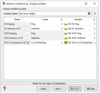
This page is only available if the Use existing kriging results option has been checked on the first page. The objective is to inform the different variables calculated from a previous kriging.

Variable Pattern: A pattern to describe the names of the Kriged variables on panels. The table immediately below this pattern shows the list of required variables:
- The kriged grade estimated,
- The dispersion variance of the kriged values (variance of Z*),
- In case of multivariate estimation, the covariance between the main and the secondary kriged estimates.
If you set the pattern to match the naming convention of the variables, then clicking the bulb in the 'Variable' cell will automatically populate the table with the kriging variable names.

In the screenshot below, the Kriged variables were created with output pattern "%method-%context-%var-%label" in the Kriging tool (the default pattern with an empty context), which creates variable names of the form "OK-Fe-Krig". That is why, we set the pattern in the UC window to "OK-%var-%label".

UC Neighborhood

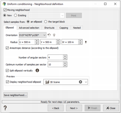
This page is skipped if the Use existing kriging results option has been checked on the first page.

You may specify a Moving neighborhood (by checking the corresponding option), either a New neighborhood or an Existing one, which uses a selection of the dataset. Parameters of this neighborhood has been defined in the Neighborhood Parameters Definition dialog area. You can press the Print button to check the relevant parameters of the neighborhood (sent in the Messages window). The created neighborhood can be saved through the Save neighborhood button (this action will be stored in batch).

If the Moving neighborhood option is not checked, a Unique neighborhood, which uses all data for every output target, will be defined.

UC Parameters

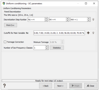
The kriging involved at the first step is a block kriging. The blocks (which correspond to the panels) need to be discretized. The number of discretization points must be sufficient to approximate correctly the mean covariance over the block. If this number is too large, the kriging will be more time consuming. The optimal number of discretization points depends on the ranges of the variogram model and on the block size. The Block Discretization parameters are required if the Block Simulations (Discretized) Mode has been chosen in the previous page. This option is available in the case of block simulations on a Grid file.

If the estimation consists in producing the optimal average value of a variable over a target block (v), the average covariance between the data point and the target cell (C_αv) as well as the average covariance of the cell (C_vv) have to be calculated. Because it is not always possible to calculate this value mathematically, the program calculates it using a discretization of the block:

where di is a discretization point and d_j a randomised point.

The block is regularly discretized according to the Discretization Steps Number NU, NV and NW. In this case, we define in how many cells we want to discretize the original block. To help you choosing the best discretization parameters, an automatic discretization is defined. This automatic value is calculated by testing different discretization steps, starting to (3,3,1) to (14,14,1). We stop to test the discretization until this one gives a covariance close to the "true" block covariance (i.e. <0.01).

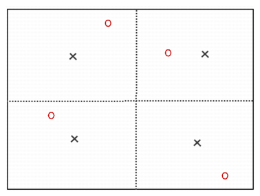
This picture shows a block discretization of two by two. Red circles correspond to random set of d_j and black crosses to the centered points di.

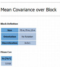
Print Cvv: To compute the average covariance of the block (C_vv), a second set of points is randomly and independently moved along X,Y and Z (50 points are selected). Of course the moving distance in a direction is smaller than the size of the block along the same direction divided by twice the number of discretizations along this direction. These moved points are only used to compute C_vv. By clicking the button, the 10 first C_vv results will be printed in the Messages window. The C_vv is also printed at the end of the Uniform Conditioning.

Click Edit to pop up the Value Definition window and customize the list of cutoffs.

Optionally, the Tonnage Correction may be activated. This option guarantees the tonnage is not below than a minimum and not greater than 1.

Note: As Uniform Conditioning may produce some results like very small total tonnages or metal tonnages, you can perform automatic corrections by selecting the Tonnage Correction option. This correction is not recommended, unless you get many inconsistencies in the mean grades versus the cutoff grades with information effect.

Number of Iso-Frequency Classes: The discrete gaussian model which allows the calculations requires transforming the kriged panel grades into gaussian values. This transformation is achieved by means of an anamorphosis function derived from the point anamorphosis and leading to the dispersion variance of the (co)kriged panels. Unlike the block anamorphosis function, the panel anamorphosis is not calculated beforehand. It is calculated when running the Uniform Conditioning and can be adapted to local dispersion variances of the panels; this is the purpose of this step. These dispersion variances will be chosen by comparing the local dispersion variance read in the grid file to the dispersion variance of fixed class intervals. These classes are obtained by assigning the dispersion variances of the (co)kriged panels for the main variable to iso-frequency classes (each class contains the same number of panels). The choice of the number of classes will obviously change the results:

if it corresponds to the total number of panels each panel will have its own panel anamorphosis with the risk of inconsistencies. For instance the dispersion variance of panels can be larger than the dispersion variance of blocks. In this case, a warning message is issued and the kriging step should be checked.
if you choose one class, the same panel anamorphosis will be used for each panel based on the average value of variances and covariances.

The final dispersion variance value chosen for one panel will be then the mean value of the corresponding iso-frequency class.

Note: If for a given class S/r > rho_v_vk (see below Statistics) there is an inconsistency. Automatically, this class and the subsequent ones are removed, the calculation continues with a reduced number of classes and an error message is printed at the end of the run.

Statistics

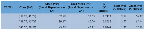
Statistics may be calculated from the dispersion variances of the kriged grade estimates (variance of Z*). The dispersion variances are ordered in a given number of iso-frequency classes. For each class, the following values are calculated:

Mean is the mean value of the dispersion variances of the grade estimates (i.e. the mean value of variance of Z*).
Used Mean is the same mean value corrected from a sill effect (difference between the variogram model sill and the variance of the data).
S is the Kriged Panel Support Correction derived from the previous value.
rho_1Vk-2Vk is the correlation coefficient between the gaussian kriged panel grade of one secondary variable with the main variable. Of course, when the secondary variable corresponds to the main variable, the correlation is equal to 1.

Kriged Panel Support Correction(S) for each variable and each class (defined on variable FE2O3)

UC Errors

A variable containing an error code is also stored in the Panel Grid File. This variable is a categorical variable indicating whether the Uniform conditioning is successful or not. The possible categories are:

Success: Uniform Conditioning is successful for that panel.
Q or T Corrected: The software corrected the grade tonnage curves, because we had inconsistencies in the QT curves (like the tonnage for the cutoff 0 is different from 1, or the grade tonnage curve is not decreasing).
Grade Inconsistency: The information effect is activated and we have an inconsistency in the grade mean (M = Q/T) or if the grade mean is below the cutoff or if the mean grade curve is decreasing (when the cutoff increases).
Relative Error too High: The curves are consistent but Q(0) is not equal to the estimated value.
Gaussian Outside Interval: When Tonnage Correction option is active, it indicates the backtransformation of the panel's Kriged Value was not possible because the value falls outside the authorized [Zmin, Zmax] interval of the model. All block/SMU values within such a panel are considered equal to Kriged panel value Z, which ensures that grades remain consistent with the model.
N/A: The result is not available either because the panel is masked-off or the kriging failed (neighborhood rules are not satisfied).

Note: When codes Relative Error too High or Gaussian Outside Interval are encountered, it is advised to run Uniform Conditioning once more without Tonnage Correction and to check whether this impacts the amount of panels which are assigned a warning code. Often the number of such panels will decrease, if the inconsistencies were due to the tonnage correction.

Note: Please note that the error code is only an indicator - just a warning - which may highlight a conflict between the kriged grades and the anamorphosis model. In such case, one would get a large proportion of panels with an error code (2, 3 or 4). When only a few panels are tagged with error codes, the resulting (Q,T,M) variables may be used safely.

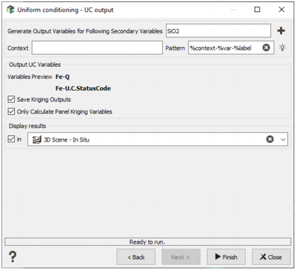
Output

Generate Output Variables for following Secondary Variables: By default, we will store the results associated to each data variable specified by the Input Geostatistical Set. Click on the to edit the variables list to deselect secondary variables whose results you do not wish to store.
The objective of the Pattern (and Context) parameter is to help the definition of output results names. It will serve as a basename for each Q/T/M result which will be stored in a macro variable whose indices will correspond to the different cutoff values. You can edit this pattern to modify it and define the name of your choice. Click on to retrieve the default pattern: %context-%var-%label
The Variables Preview enables you to see the final name associated to the output results (for the main variable).
Save Kriging Outputs: Tick this option to store the kriged grade estimated as well as the dispersion variance produced by the uniform conditioning. This option is not available if the Use existing kriging results option has been checked on the first page.
Only Calculate Panel Kriging Variables: This option enables to calculate the same variables as in Kriging Neighborhood Analysis (KNA) on the Panel grid, without having to wait for the full UC (and LUC) calculation. With those variable statistics, you can easily modify the neighborhood. And do the UC/LUC calculation when the KNA statistics will be OK. When activating the option, QTM variables and LUC variables won't be calculated.
Enter here a New Neighborhood Name to save your neighborhood parameters and use them in a second run or in another panel.
Select the Display Results toggle to display the result of your uniform conditioning (or LUC depending on the option) in a defined scene (2D or 3D) at the end of the run.