|
|
Gridding controls used in contouring |

Generate Contours - Gridding
To access this dialog:
-
From the Data page of the Generate Contours wizard, fill out the fields and click Next. The Gridding page is displayed.
The Gridding panel is part of the contour generation function. It is used to set up parameters required to generate the output data (grid model, contours and/or surface).
The same panel is used when generating contours from points and drillhole intercepts. If a distance-from-sample map is being created, some functions are not available.
You can choose to calculate the size of your output grid based on either your current loaded/specified data or you can choose a custom area.
For more general information on contouring, including examples and procedures involving the gridding page, see:
- Contours from Points
- Contours from Intercepts
- Procedure: Grade Contours from Points
- Procedure: Elevation Contours from Points
- Procedure: Distance-from-Sample Contours
- Example: Contours from Intercepts
- Related Topics, below
When you have completed entering details for the contour gridding,
click Next to view the Output
Data panel.
|
|
Use the Back and Next buttons to access functionality in the Generate Contours wizard. Once you have completed setting you your parameters, click Finish to create your output object(s). Once data has been generated, your previous settings can be retrieved in a subsequent session using Restore. |
Field Details:
Extents:
This section of the dialog allows you to control the 'hull' of your output data.
Use Data Extents: select this option to generate grid, contours and/or wireframe data based on the current dimensions of your loaded/specified input data. You can either select this or the Custom option (see below). You can specify an extra Margin if you wish (see below).
Margin: The Margin setting is the amount by which the contours (and surface) are extended beyond the original data hull. The Margin is added to the data extents shown in the read-only dimension fields below.
Custom: select this option to display the current data extents (or last modified values) as editable fields.
The generated grid always uses the Min and Max values regardless or any intermediate changes to margin (although the actual grid max may be rounded up to the next whole cell size).
Resolution:
The Resolution area lets you define the grid cell size or number of grid cells used in the output grid model (if you aren't creating one, you can ignore this section). This is like the NGRID parameter used in implicit modelling commands; it increases or decreases the distance between grid points.
-
If setting the Cell Width and Height, higher numbers will reduce the inter-point distance of the grid.
-
If setting the number of Cells Across and Up, higher numbers increase the distance.
Consider the following
example images, where the top image shows the wireframe (with highlighted
edges) output using a coarse 10 x 10 resolution and the lower image
shows a 100 x 100 resolution output: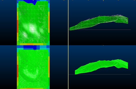
Estimation:
Estimation parameters determine how the surface is generated between points.
Algorithm (not displayed with generate-distance-contours command): select the gridding method to be used during contour calculation, using one of the following:
-
Distance Weighted Average: the estimate is the average of sample values used by weighting the inversely to the square of their distance from the node.
This method uses a distance weighted average to determine points from surrounding values. All points around a grid cell are used in deriving an estimate at the grid node. A weight is assigned to each value inversely proportional to the square of the distance of the data point from the grid cell. This method has a tendency to smooth out localized highs and lows but is fairly accurate under a wide range of conditions (Lam, 1986).
One limitation is that estimates are bounded by the extrema in sampled values, and the radial symmetry imparted tends to obscure the effect of linear features such as ridges or valleys (Watson and Phillip, 1985). Good surface elevation results are obtained when poor spatial correlation is an issue (Falivene et al, 2009). -
Minimum Curvature: this is also an inverse distance weighted average method, but also uses slope information at the node being estimated.
Minimum curvature works by fitting the surface with the smallest change in slope (the “minimum curve”) to the data set. This provides a conservative estimate of the surface modeled by the data.
It preserves continuity, or in other words, rate of change of slope (Briggs, 1974). Surfaces may have large oscillations and extraneous inflection points (Smith and Wessel, 1990). Generally this method gives good results for all types of data, and is particularly adept at modelling surface elevations and reservoir thickness (Falivene et al, 2009).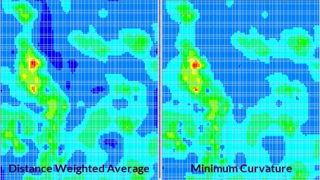
-
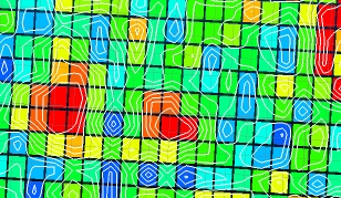
Trend Surface: this option uses a polynomial projection to interpolate the grid, wireframe and strings from known point positions. You can choose the Polynomial order from 1-6. The order of the polynomial can be determined by the number of fluctuations in the data or by how many bends (hills and valleys) appear in the curve. An Order 2 polynomial trendline generally has only one hill or valley. Order 3 generally has one or two hills or valleys. Order 4 generally has up to three.
As a rule of thumb, a polynomial fit will sacrifice close adherence to precise sample positions in favour of establishing a realistic data trend. This can be useful when extrapolating to a contact boundary that lies outside the main body of data, for example.
For example, a 1st order polynomial generated across a set of 3D data points will be a flat mean plane, whereas a 2nd order polynomial may looks something closer to this (cross section of 3D data shown):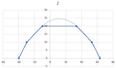
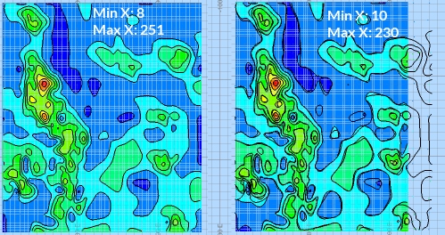
Consider a 3D version of the above section, where the scene contains a series of points arranged in a concentric square arrangement with increasing Z values towards the centre of data, e.g.: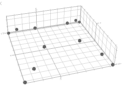
The image on the left below represents a first order polynomial, and a 2nd order polynomial on the right: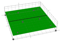
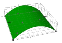
And a 3rd order...: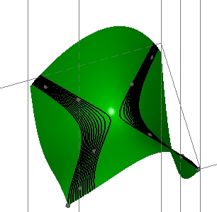
Here's a comparison of contoured surface (only) output for the same input data and settings other than the estimation method. Specifically, it is a comparison of the Minimum Curvature method and the Trend Surface method: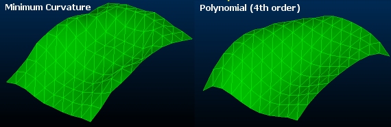
Estimation (not displayed with generate-distance-contours command nor for Trend Surfacae estimations): select the interpolation method. The interpolation method for a grid is the method used to interpolate high resolution values within grid model cells
As a general rule, this should be [Slope] for
smoothly varying surfaces or [Slope Curvature] for surfaces in which
sharp breaks in slope are to be retained.
For the majority of cases, the default [Slope] setting is fine.
Smoothing (not displayed with generate-distance-contours command nor for Trend Surface estimations): there are several smoothing options available with this tool. As a general rule, for the same number of passes the bi-harmonic will smooth the grid less than either the Average or the Bartlett. The average filter will result in less smoothing than the Bartlett 5, but may give smoother results than the Bartlett3.
The Bartlett5 and 7 are commonly used to smooth velocity maps as they may require a lot of smoothing. The other filters are used where you only want to remove some high frequency jitter in the data.
Select an option from the drop-down list:
-
Biharmonic: this type of smoothing uses a Forced Bi-harmonic operator; results from the previous convergent gridding pass are kept and the new solution is forced to have the same values at the same points as the previous iteration. In other words, data values are honoured in this type of smoothing and it is a very mild form of smoothing.
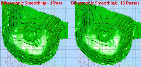
A biharmonic filter reduces net surface curvature whilst retaining all features which are larger than the size of 1 grid cell. The smoothing honours fault polygons. -
Average: A three-point filter is applied with the following weightings:
0 1 0
1 4 0
0 1 0
The filter is applied to a grid node by multiplying the input values by the filter weights, summing and then dividing by the total of the filter value. -
Bartlett 3/5/7: There is a choice of a 3, 5 or 7 point filter operator. The filter is applied to a grid node by multiplying the input values by the filter weights, summing and then dividing by the total of the filter value. [Bartlett7] will give the smoothest result.
They have the following weightings:
| 3-point |
1 |
2 |
1 |
|
|
|
|
|
2 |
4 |
2 |
|
|
|
|
|
|
1 |
2 |
1 |
|
|
|
|
|
| 5-point |
1 |
2 |
3 |
2 |
1 |
|
|
|
2 |
4 |
6 |
4 |
2 |
|
|
|
|
3 |
6 |
9 |
6 |
3 |
|
|
|
|
2 |
4 |
6 |
4 |
2 |
|
|
|
|
1 |
2 |
3 |
2 |
1 |
|
|
|
| 7-point |
1 |
2 |
3 |
4 |
3 |
2 |
1 |
|
2 |
4 |
6 |
8 |
6 |
4 |
2 |
|
|
3 |
6 |
9 |
12 |
9 |
6 |
3 |
|
|
4 |
8 |
12 |
16 |
12 |
8 |
4 |
|
|
3 |
6 |
9 |
12 |
9 |
6 |
3 |
|
|
2 |
4 |
6 |
8 |
6 |
4 |
2 |
|
|
1 |
2 |
3 |
4 |
3 |
2 |
1 |
|
|
Grids can be smoothed in a variety of other ways:
|
Use Search Ellipse (not displayed with generate-distance-contours command nor for Trend Surface estimations): select this option if you wish to generate a model to consider an anisotropic trend within the data. The axes of the 2D search ellipse will determine the predilection for each sample point to influence the grid in a given direction (showing a stronger influence in the major axis of the ellipse.
The Rotation represents the azimuth of the 2D ellipse. The Minor axis length and Major axis length should be set to a value that represents the extent of anisotropy within the data set (only one ellipse can be defined for each contouring run).
The Min. samples field is used to indicate how many samples should be within the ellipse (when centered at each sample point) in order to influence the contouring results. Higher sample numbers will lower the tendency for anisotropy to be considered.
|
|
Contouring commands are scriptable. You can find out more using this Knowledge Base Article. |
Copyright © Datamine Corporate Limited
JMN 20045_00_EN
Some information in this article has been provided courtesy of Petrosys Inc. All rights reserved. Petrosys is a registered trademark and a wholly-owned subsidiary of Datamine Corporate Limited.